Atmospheric and Climate Sciences
Vol.3 No.3A(2013), Article ID:34973,12 pages DOI:10.4236/acs.2013.33A002
A Simulation Study of the Effect of Geomagnetic Activity on the Global Circulation in the Earth’s Middle Atmosphere
Polar Geophysical Institute, Kola Scientific Center of the Russian Academy of Sciences, Apatity, Russia
Email: *mingalev@pgia.ru
Copyright © 2013 Igor Mingalev et al. This is an open access article distributed under the Creative Commons Attribution License, which permits unrestricted use, distribution, and reproduction in any medium, provided the original work is properly cited.
Received April 24, 2013; revised May 26, 2013; accepted June 2, 2013
Keywords: Middle Atmosphere; Global Circulation; Numerical Simulation
ABSTRACT
To investigate how geomagnetic activity affects the formation of the large-scale global circulation of the middle atmosphere, the non-hydrostatic model of the global wind system of the Earth’s atmosphere, developed earlier in the Polar Geophysical Institute, is utilized. The model produces three-dimensional global distributions of the zonal, meridional, and vertical components of the wind velocity and neutral gas density in the troposphere, stratosphere, mesosphere, and lower thermosphere. Simulations are performed for the winter period in the northern hemisphere (16 January) and for two distinct values of geomagnetic activity (Kp = 1 and Kp = 4). The simulation results indicate that geomagnetic activity ought to influence considerably on the formation of global wind system in the stratosphere, mesosphere, and lower thermosphere. The influence on the middle atmosphere is conditioned by the vertical transport of air from the lower thermosphere to the mesosphere and stratosphere and vice versa. This transport may be rather distinct under different geomagnetic activity conditions.
1. Introduction
An investigation of the dynamical processes in the Earth’s atmosphere is a very important problem. It is well known that the atmospheric processes influence considerably on the human activity and health. Unfortunately, modern scientific facility does not allow somebody to measure the momentary global three-dimensional wind system of the Earth’s atmosphere. However, to investigate the planetary wind system of the Earth’s atmosphere, mathematical models may be utilized.
During the last three decades, several general circulation models of the lower and middle atmosphere have been developed (e.g., see [1-11]). It can be noticed that the existing general circulation models of the lower and middle atmosphere may be successfully utilized for simulation of the slow climate changes.
Not long ago, in the Polar Geophysical Institute (PGI), the non-hydrostatic model of the global neutral wind system in the Earth’s atmosphere has been developed [12,13]. This model enables to calculate three-dimensional global distributions of the zonal, meridional, and vertical components of the neutral wind at levels of the troposphere, stratosphere, mesosphere, and lower thermosphere, with whatever restrictions on the vertical transport of the neutral gas being absent. This model has been utilized in order to simulate the global circulation of the middle atmosphere for conditions corresponding to different seasons [12-15] and to investigate numerically how solar activity affects the formation of the large-scale global circulation of the mesosphere and lower thermosphere [16]. The purpose of the present work is to continuer these studies and to investigate numerically, using the non-hydrostatic model of the global neutral wind system, developed earlier in the Polar Geophysical Institute, how geomagnetic activity affects the formation of the large-scale global circulation of the stratosphere, mesosphere, and lower thermosphere.
2. Mathematical Model
In the present study, the non-hydrostatic model of the global neutral wind system in the Earth’s atmospheredeveloped earlier in the PGI [12,13], is utilized. This model produces three-dimensional global distributions of the zonal, meridional, and vertical components of the neutral wind and neutral gas density in the troposphere, stratosphere, mesosphere, and lower thermosphere. The peculiarity of the utilized model consists in that the internal energy equation for the neutral gas is not solved in the model calculations. Instead, the global temperature field is assumed to be a given distribution, i.e. the input parameter of the model, and obtained from the NRLMSISE-00 empirical model [17]. Moreover, in the model calculations, not only the horizontal components but also the vertical component of the neutral wind velocity is obtained by means of a numerical solution of a generalized Navier-Stokes equation for compressible gas, so the model is non-hydrostatic.
The mathematical model, utilized in the present study, is based on the numerical solution of the system of equations containing the dynamical equation and continuity equation for the neutral gas. For solving the system of equations, the finite-difference method is applied. The dynamical equation for the neutral gas in vectorial form can be written as
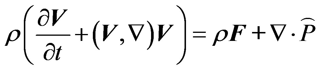 (1)
(1)
where  is the neutral gas density,
  is the neutral wind velocity,
  is the acceleration comprising the gravity acceleration, Coriolis acceleration, acceleration of translation, and acceleration due to elastic collisions with the ion gas, and
  is the total stress tensor. The latter tensor can be decomposed as follows:
 (2)
(2)
where ![]() is the pressure,
is the pressure,  is the unit tensor, and
  is the extra stress tensor whose components are given by the rheological equation of state or the law of viscous friction. A spherical coordinate system rotatable together with the Earth is utilized in model calculations. Therefore, from the dynamical equation, Equation (1), momentum equations for the zonal, meridional, and vertical components of the neutral gas velocity may be derived. These equations include not only the pressure gradients but also partial derivatives of components of the extra stress tensor,
 . The latter tensor is composed of a Newtonian part,
  , and a complementary part,
  , namely,
 (3)
(3)
the former tensor,  , is given by the well-known Newton’s law of viscous friction,
 (4)
(4)
where  is the coefficient of molecular viscosity, whose dependence on the temperature is assumed to obey the Sutherland’s law, and
  is the tensor defined as
 (5)
(5)
where  is the strain rate tensor and
  denotes the trace of a tensor. The complementary stress tensor,
  , is supposed to be conditioned by a small-scale turbulence having the scales equal and less than the steps of the finite-difference approximations. It is assumed that this tensor represents the effect of the turbulence on the mean flow and is given by an expression, analogous to the Newton’s law of viscous friction, Equation (4), with the scalar coefficient of viscosity,
  , being replaced by three distinct coefficients describing the eddy viscosities in the directions of the basis vectors of the utilized spherical coordinate system. For computing the eddy viscosities, the turbulence theory of Obukhov [18] is applied.
Thus, the momentum equations for the zonal, meridional, and vertical components of the neutral gas velocity acquire ultimately a form of a generalized Navier-Stokes equation for compressible gas on scales which are more than the steps of the finite-difference approximations, with the effect of the turbulence on the mean flow being taken into account by using an empirical subgrid-scale parameterization. The steps of the finite-difference approximations in the latitude and longitude directions are identical and equal to 1 degree. A height step is non-uniform and does not exceed the value of 1 km.
The simulation domain is the layer surrounding the Earth globally and stretching from the ground up to the altitude of 126 km at the equator. Upper boundary conditions provide the conservation law of mass in the simulation domain. The Earth's surface is supposed to coincide approximately with an oblate spheroid whose radius at the equator is more than that at the pole. More complete details of the utilized model may be found in the studies of I. Mingalev, and V. Mingalev, [12] and Mingalev et al. [13].
3. Presentation and Discussion of Results
The utilized mathematical model of the global neutral wind system can be used for different seasonal, solar cycle, and geomagnetic conditions. In the present study, simulations are performed for the winter period in the northern hemisphere (16 January) and for conditions corresponding to moderate 10.7 cm solar flux (F10.7 = 101). To investigate the influence of geomagnetic activity on the global circulation of the atmosphere, we made calculations for conditions corresponding to two different values of geomagnetic activity: low and considerable, namely, Kp = 1 and Kp = 4. The variations of the atmospheric parameters with time were calculated until they become stationary. The steady-state distributions of the atmospheric parameters were obtained on condition that inputs to the model and boundary conditions correspond to 10.30 UT. The temperature distributions, corresponding to this moment, were calculated using the NRLMSISE-00 empirical model [17].
It turns out that atmospheric temperatures, calculated with the help of the NRLMSISE-00 empirical model for two distinct values of geomagnetic activity (Kp = 1 and Kp = 4), are very similar below approximately 80 km, while, above this altitude, they may be rather different. Figure 1 shows the global distributions of the atmospheric temperature at 50 km altitude, obtained from the NRLMSISE-00 empirical model for 16 January, UT = 10.30 and calculated for two distinct values of geomagnetic activity: Kp = 1 and Kp = 4. It is seen no distinctions between the results obtained for two different values of geomagnetic activity.
On the contrary, from Figure 2, in which the global distributions of the atmospheric temperature at 110 km altitude are present, one can see that differences between temperatures, obtained for two considered values of geomagnetic activity, can achieve a few tens of degrees at identical points of the globe. Thus, the application of the NRLMSISE-00 empirical model shows that the influence of level of geomagnetic activity on the global distribution of the atmospheric temperature ought to be absent at altitudes of the troposphere, stratosphere, and mesosphere, while this influence ought to be appreciable at altitudes of the lower thermosphere for the winter period in the northern hemisphere.
Distributions of the atmospheric parameters, calculated with the help of the mathematical model and obtained for 16 January for two different values of geomagnetic activity, are shown in Figures 3 - 12. The results of modeling illustrate both common characteristic features and distinctions caused by different values of geomagnetic activity.
The calculated global distributions of the atmospheric parameters display the following common features. At levels of the stratosphere, mesosphere, and lower thermosphere, the horizontal and vertical components of the wind velocity are changeable functions of latitude and longitude. Maximal absolute values of the horizontal and vertical components of the wind velocity are larger at higher altitudes. The horizontal domains exist where the steep gradients in the horizontal velocity field take place. The horizontal wind velocity can have various directions which may be opposite at the near points. Moreover, the horizontal domains exist in which the vertical neutral wind component has opposite directions. The horizontal
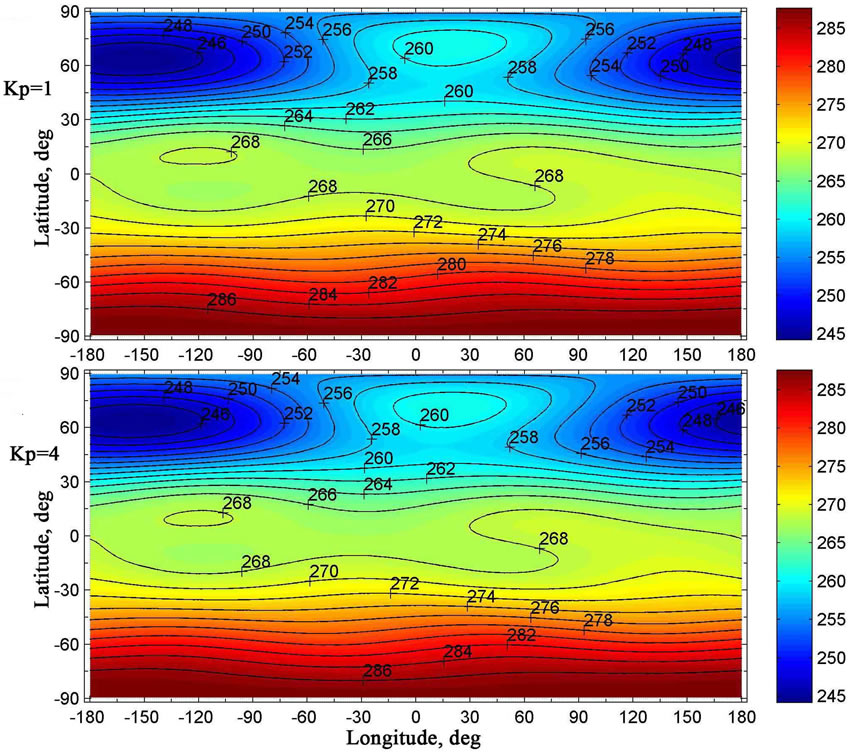
Figure 1. The global distributions of the atmospheric temperature (K) at 50 km altitude, obtained from the NRLMSISE-00 empirical model for 16 January, UT = 10.30 and calculated for two distinct values of geomagnetic activity: Kp = 1 (top panel) and Kp = 4 (bottom panel).
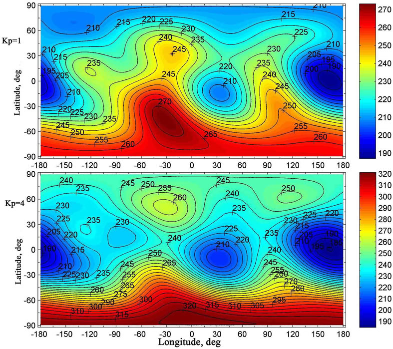
Figure 2. The global distributions of the atmospheric temperature (K) at 110 km altitude, obtained from the NRLMSISE-00 empirical model for 16 January, UT = 10.30 and calculated for two distinct values of geomagnetic activity: Kp = 1 (top panel) and Kp = 4 (bottom panel).
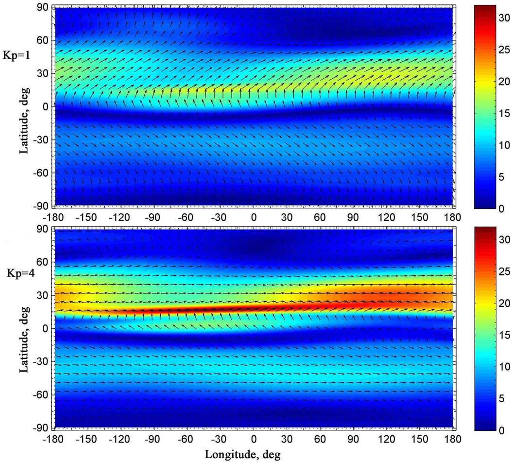
Figure 3. The global distributions of the vector of the simulated horizontal component of the neutral wind velocity at the altitude of 10 km, obtained for 16 January and calculated for two distinct values of geomagnetic activity: Kp = 1 (top panel) and Kp = 4 (bottom panel). The colouration of the figures indicates the module of the velocity in m/s.

Figure 4. The same as in Figure 3 but at the altitude of 20 km. The colouration of the figures indicates the module of the velocity in m/s.
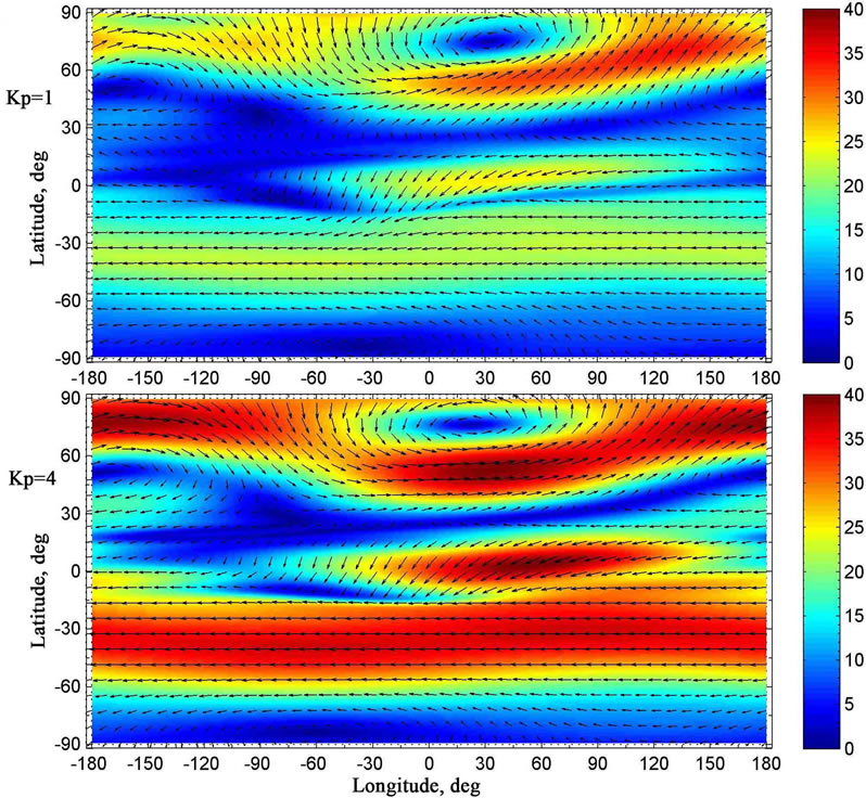
Figure 5. The same as in Figure 3 but at the altitude of 30 km. The colouration of the figures indicates the module of the velocity in m/s.
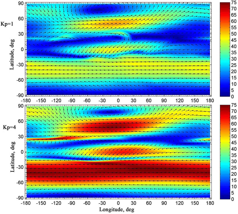
Figure 6. The same as in Figure 3 but at the altitude of 50 km. The colouration of the figures indicates the module of the velocity in m/s.
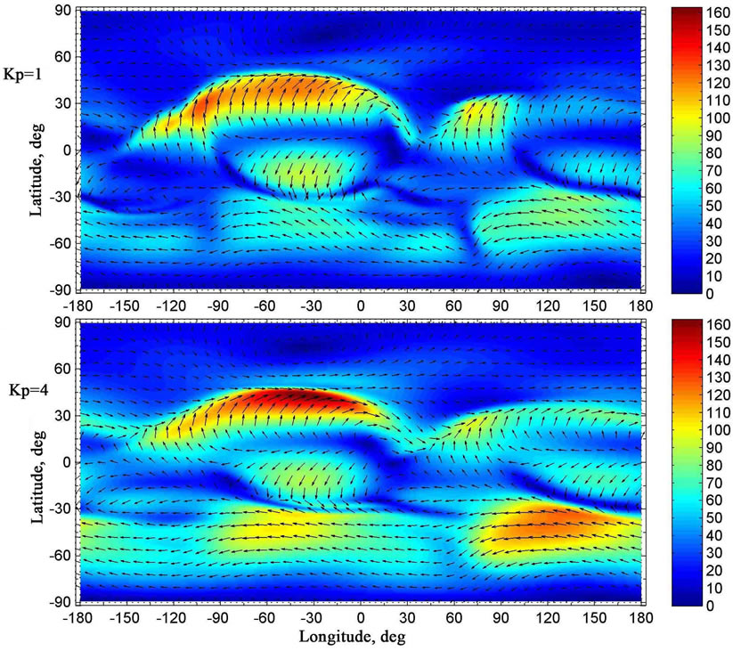
Figure 7. The same as in Figure 3 but at the altitude of 70 km. The colouration of the figures indicates the module of the velocity in m/s.
domains, where the vertical neutral wind component is upward, have a great length and large width, as a rule. Unlike, the horizontal domains, where the vertical neutral wind component is downward, have a large length and little width. Usually, the latter domains have a configuration like a long narrow band and coincide, as a rule, with the regions, where the steep gradients in the horizontal velocity field take place. Maximal absolute values of the upward vertical wind component are less than the maximal module of the downward vertical wind component. At levels of the mesosphere, the horizontal wind velocity can achieve values of more than 150 m/s.
It is well known from numerous observations that the global atmospheric circulation can contain sometimes so called circumpolar vortices that are the largest scale inhomogeneities in the global neutral wind system. Their extent can be very large, sometimes reaching the latitudes close to the equator. It is known that circumpolar vortices are often formed at heights of the stratosphere and mesosphere in the periods close to summer and winter solstices. The circumpolar cyclone arises in the northern hemisphere under winter conditions, while the circumpolar anticyclone arises in the southern hemisphere under summer conditions.
From the numerically obtained results for winter period in the northern hemisphere, we can see that, at levels of the stratosphere and mesosphere, the motion of the neutral gas in the northern hemisphere is primarily eastward, so a circumpolar cyclone is formed (Figures 4 - 7). It can be noticed that the center of the northern cyclone may be displaced from the pole. Simultaneously, the motion of the neutral gas is primarily westward in the southern hemisphere at levels of the stratosphere and mesosphere, so a circumpolar anticyclone is formed for summer period of the southern hemisphere (Figures 4 - 7). It can be seen that the circumpolar vortices of the northern and southern hemispheres, numerically simulated in the present study at levels of the stratosphere and mesosphere, correspond qualitatively to the global circulation, obtained from observations.
Let us consider simulation results, obtained for distinct values of magnetic activity, and their distinctions. It is easy to see that, at levels of the lower thermosphere, maximal absolute values of the horizontal components of the wind velocity, obtained for low geomagnetic activity, are less than those, obtained for considerable geomagnetic activity (Figure 9). It is obvious that these distinctions are conditioned by the differences of the temperature distributions, obtained for two distinct values of geomagnetic activity (Figure 2).
It can be seen that, at levels of the upper troposphere, stratosphere, and mesosphere, the global distributions of the vector of the simulated horizontal component of the neutral wind velocity, calculated for two distinct values of geomagnetic activity, are rather different (Figures 3 - 7). These differences can not be explained by the distinctions of the temperature distributions because of the absence of these distinctions below approximately 80 km, as was noted earlier. The simulation results indicate that the effect of geomagnetic activity on the global circulation of the atmosphere below 80 km is conditioned by the vertical transport of air from the thermosphere to the lower levels and vice versa. As can be seen from Figures 10 - 12, such vertical transport does exist. This transport may be rather distinct under different geomagnetic activity conditions. It can be noticed that the utilized mathematical model is able to simulate this vertical transport due to the fact that the model is non-hydrostatic.
Thus, the simulation results indicate that geomagnetic activity ought to influence considerably on the formation of global neutral wind system not only in lower thermosphere, but also in the mesosphere, stratosphere, and upper troposphere. In particular, from the results shown in Figures 5 - 7, one can see that the horizontal wind velocity in the circumpolar cyclone of the northern hemisphere, obtained for low geomagnetic activity, is less than that, obtained for considerable geomagnetic activity. Similarly, the horizontal wind velocity in the circumpolar anticyclone of the southern hemisphere, obtained for low geomagnetic activity, is less than that, obtained for considerable geomagnetic activity.
The level of geomagnetic activity can influence not only on the magnitude of the horizontal wind velocity in the circumpolar cyclone of the northern hemisphere, but also on the vertical dimension of this cyclone. From the results shown in Figure 4, one can see that the altitude of the lower edge of this circumpolar cyclone depends of the level of geomagnetic activity. Pronounced circumpolar cyclone is present in the northern hemisphere at 20 km altitude under considerable geomagnetic activity, with its center being displaced from the pole. On the contrary, under low geomagnetic activity, the pronounnced circumpolar cyclone is absent in the northern hemisphere at 20 km altitude (Figure 4). From Figure 5, it can be seen that the pronounced circumpolar cyclone is present in the northern hemisphere at 30 km altitude under two distinct values of geomagnetic activity.
From the obtained results, we can see that, at levels near to the stratopause, the vertical wind velocity can have opposite directions in the horizontal domains having different configurations. Maximal absolute values of the downward vertical wind component are commensurable with the maximal module of the upward vertical wind component for conditions of low geomagnetic activity. On the contrary, for conditions of considerable geomagnetic activity, maximal absolute values of the downward and upward vertical wind components can be rather different (Figure 10).
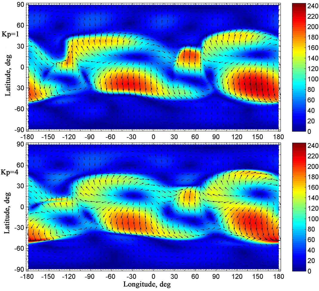
Figure 8. The same as in Figure 3 but at the altitude of 90 km. The colouration of the figures indicates the module of the velocity in m/s.
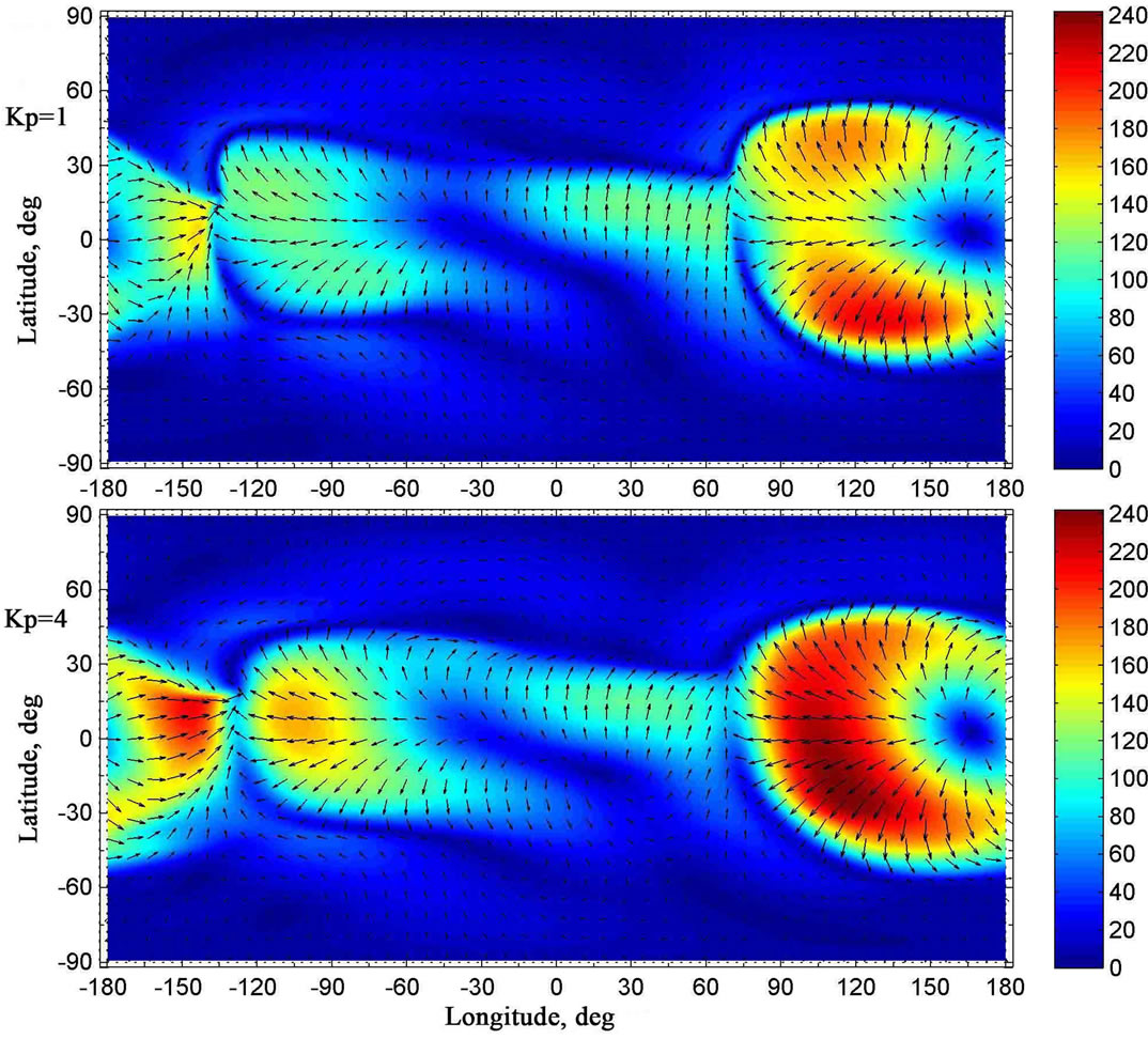
Figure 9. The same as in Figure 3 but at the altitude of 110 km. The colouration of the figures indicates the module of the velocity in m/s.
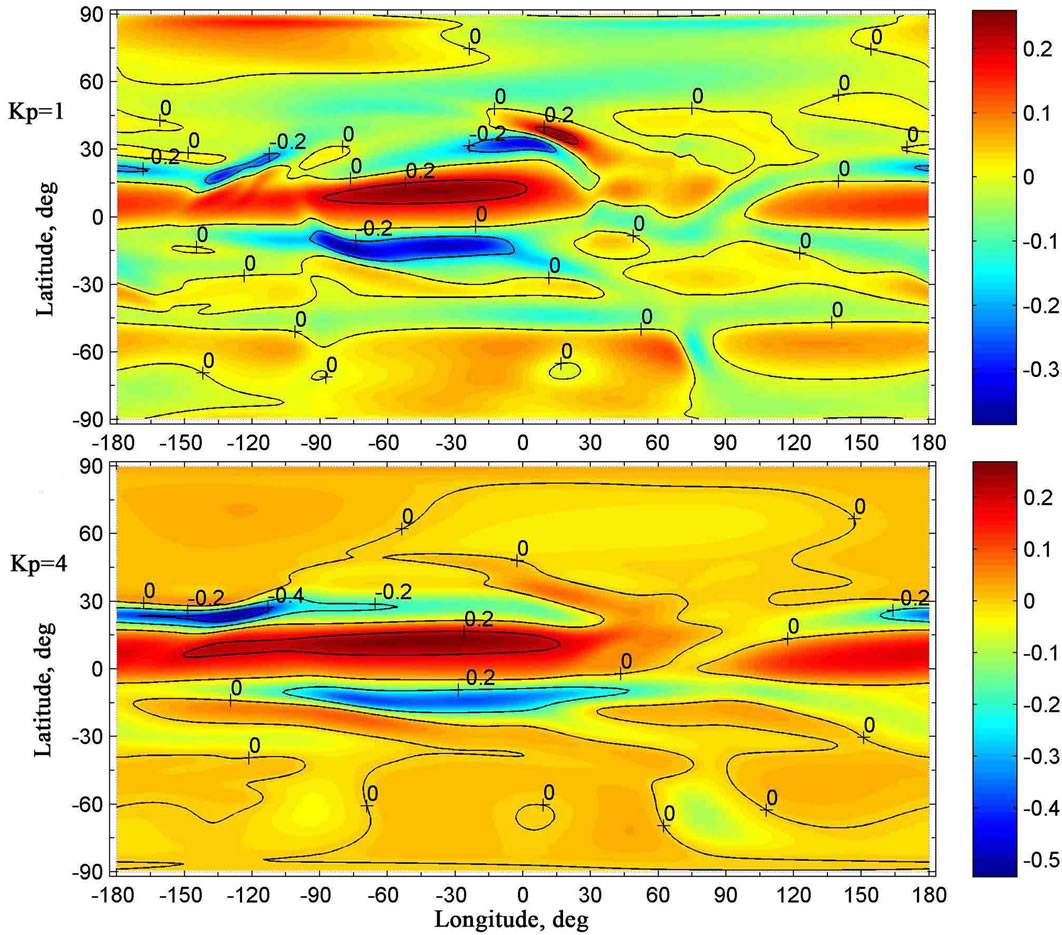
Figure 10. The global distributions of the simulated vertical component of the neutral wind velocity at the altitude of 50 km, obtained for 16 January and calculated for two distinct values of geomagnetic activity: Kp = 1 (top panel) and Kp = 4 (bottom panel). The colouration of the figures indicates the velocity in m/s, with the positive direction of the vertical velocity being upward.
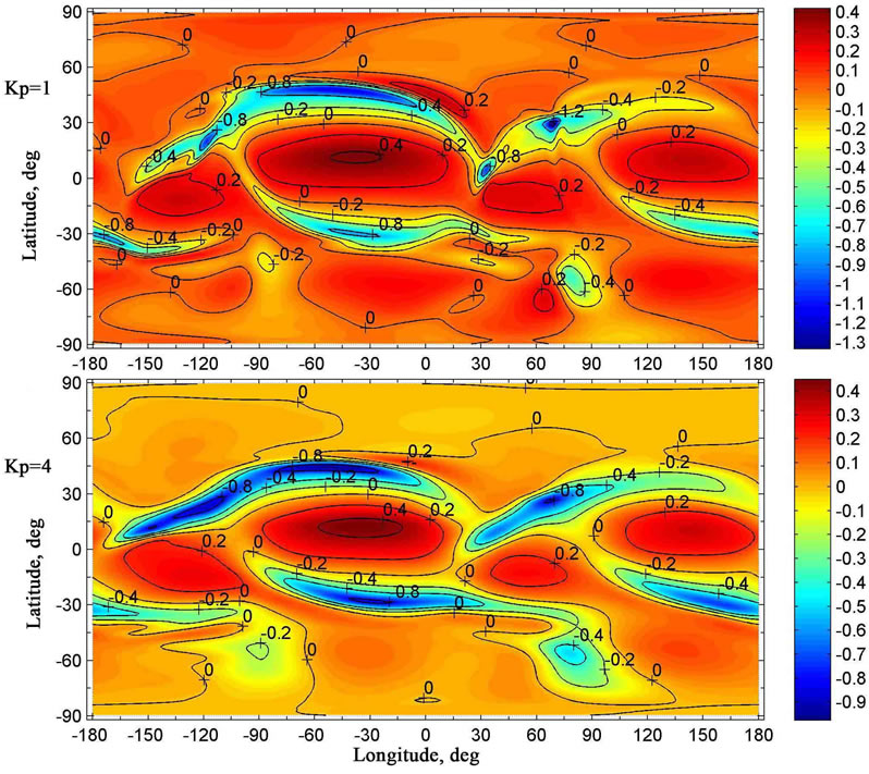
Figure 11. The same as in Figure 10 but at the altitude of 70 km. The colouration of the figures indicates the velocity in m/s, with the positive direction of the vertical velocity being upward.
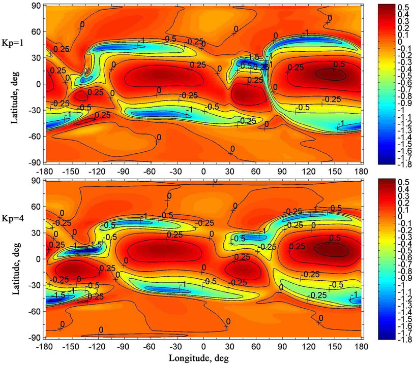
Figure 12. The same as in Figure 10 but at the altitude of 90 km. The colouration of the figures indicates the velocity in m/s, with the positive direction of the vertical velocity being upward.
The simulation results indicate that, at levels of mesosphere at latitudes close to the equator, the distributions of the vector of the horizontal component of the neutral wind velocity, calculated for two distinct values of geomagnetic activity, are qualitatively similar (Figures 4 - 6). However, the maximal module of the horizontal wind velocity, obtained for low geomagnetic activity, is less than that, obtained for considerable geomagnetic activity, at latitudes close to the equator.
4. Summary and Conclusions
To investigate how geomagnetic activity affects the formation of the large-scale global circulation of the middle atmosphere, the non-hydrostatic model of the global wind system of the Earth’s atmosphere, developed earlier in the Polar Geophysical Institute, is utilized. The model produces three-dimensional global distributions of the zonal, meridional, and vertical components of the wind velocity and neutral gas density in the troposphere, stratosphere, mesosphere, and lower thermosphere. The peculiarity of the utilized model consists in that not only the horizontal components but also the vertical component of the neutral wind velocity is obtained by means of a numerical solution of a generalized Navier-Stokes equation for compressible gas, so the model is non-hydrostatic. Moreover, the internal energy equation for the neutral gas is not solved in the model calculations. Instead, the global temperature field is assumed to be a given distribution, i.e. the input parameter of the model, and obtained from the NRLMSISE-00 empirical model [17].
The applied mathematical model was utilized for obtaining the steady-state distributions of the atmospheric parameters, using the method of establishment, for conditions, corresponding to moderate 10.7 cm solar flux (F10.7 = 101) for the winter period in the northern hemisphere (16 January). The distributions of the atmospheric parameters were obtained on condition that inputs to the model and boundary conditions correspond to 10.30 UT. To investigate the influence of geomagnetic activity on the global circulation of the atmosphere, calculations were made for conditions corresponding to two different values of geomagnetic activity: low and considerable, namely, Kp = 1 and Kp = 4.
The calculated global distributions of the atmospheric parameters display the common characteristic features. At levels of the stratosphere, mesosphere, and lower thermosphere, the horizontal and vertical components of the wind velocity are changeable functions of latitude and longitude. It turned out that the calculated global distributions of the horizontal wind velocity, obtained for different values of geomagnetic activity, contain large-scale circumpolar vortices of the northern and southern hemispheres. The circumpolar vortices of the northern and southern hemispheres, numerically simulated in the present study at levels of the stratosphere and mesosphere, correspond qualitatively to the global circulation, obtained from observations.
The simulation results indicate that geomagnetic activity ought to influence considerably on the formation of global neutral wind system in the stratosphere, mesosphere, and lower thermosphere. However, this influence is not straightforward.
Undoubtedly, at levels of the lower thermosphere, this influence is conditioned by the differences of the temperature distributions, obtained for various values of geomagnetic activity at these levels. However, from the simulation results obtained, we can see that the atmospheric temperature, calculated with the help of the NRLMSISE-00 empirical model, does not depend on the geomagnetic activity below approximately 80 km. Nevertheless, the effect of geomagnetic activity on the global circulation of the atmosphere below 80 km exists. This effect is conditioned by the vertical transport of air from the lower thermosphere to the mesosphere, stratosphere, and upper troposphere, eventually, and vice versa. The simulation results indicate that this vertical transport may be rather distinct under different geomagnetic activity conditions.
Thus, the influence of geomagnetic activity on the global circulation in the Earth’s middle and lower atmospheres for January conditions is a consequence of a relationship between large-scale global circulation of the lower thermosphere and large-scale planetary circulations of the middle and lower atmospheres, with the vertical transport of air playing a significant role.
It can be noticed that the utilized mathematical model was able to simulate the effect of geomagnetic activity on the global circulation in the Earth’s middle and lower atmospheres due to the fact that the model is non-hydrostatic.
5. Acknowledgements
This work was partly supported by Grant No. 13-01- 00063 from the Russian Foundation for Basic Research.
REFERENCES
- S. Manabe and D. G. Hahn, “Simulation of Atmospheric Variability,” Monthly Weather Review, Vol. 109, No. 11, 1981, pp. 2260-2286. doi:10.1175/1520-0493(1981)109<2260:SOAV>2.0.CO;2
- D. Cariolle, A. Lasserre-Bigorry, J.-F. Royer and J.-F. Geleyn, “A General Circulation Model Simulation of the Springtime Antarctic Ozone Decrease and Its Impact on Mid-Latitudes,” Journal of Geophysical Research, Vol. 95, No. 2, 1990, pp. 1883-1898. doi:10.1029/JD095iD02p01883
- P. J. Rasch and D. L. Williamson, “The Sensitivity of a General Circulation Model Climate to the Moisture Transport Formulation,” Journal of Geophysical Research, Vol. 96, No. D7, 1991, pp. 13123-13137. doi:10.1029/91JD01179
- H. F. Graf, I. Kirchner, R. Sausen and S. Schubert, “The Impact of Upper-Tropospheric Aerosol on Global Atmospheric Circulation,” Annales Geophysicae, Vol. 10, No. 9, 1992, pp. 698-707.
- P. A. Stott and R. S. Harwood, “An implicit time-stepping scheme for chemical species in a Global atmospheric circulation model”, Annales Geophysicae, Vol. 11, 1993, pp. 377-388.
- B. Christiansen, A. Guldberg, A. W. Hansen and L. P. Riishojgaard, “On the Response of a Three-Dimensional General Circulation Model to Imposed Changes in the Ozone Distribution,” Journal of Geophysical Research, Vol. 102, No. D11, 1997, pp. 13051-13078. doi:10.1029/97JD00529
- V. Y. Galin, “Parametrization of Radiative Processes in the DNM Atmospheric Model,” Izvestiya Akademii Nauk, Physics of Atmosphere and Ocean, Vol. 34, No. 3, 1997, pp. 380-389.
- A.-L. Gibelin and M. Deque, “Anthropogenic Climate Change over the Mediterranean Region Simulated by a Global Variable Resolution Model,” Climate Dynamics, Vol. 20, No. 4, 2002, pp. 327-339.
- M. Mendillo, H. Rishbeth, R. G. Roble and J. Wroten, “Modelling F2-Layer Seasonal Trends and Day-To-Day Variability Driven by Coupling with the Lower Atmosphere,” Journal of Atmospheric and Solar-Terrestrial Physics, Vol. 64, No. 18, 2002, pp. 1911-1931. doi:10.1016/S1364-6826(02)00193-1
- M. J. Harris, N. F. Arnold and A. D. Aylward, “A Study into the Effect of the Diurnal Tide on the Structure of the Background Mesosphere and Thermosphere Using the New Coupled Middle Atmosphere and Thermosphere (CMAT) General Circulation Model,” Annales Geophysicae, Vol. 20, No. 2, 2002, pp. 225-235. doi:10.5194/angeo-20-225-2002
- U. Langematz, A. Claussnitzer, K. Matthes and M. Kunze, “The Climate during Maunder Minimum: A Simulation with Freie Universitat Berlin Climate Middle Atmosphere Model (FUB-CMAT),” Journal of Atmospheric and Solar-Terrestrial Physics, Vol. 67, No. 1-2, 2005, pp. 55-69. doi:10.1016/j.jastp.2004.07.017
- I. V. Mingalev and V. S. Mingalev, “The Global Circulation Model of the Lower and Middle Atmosphere of the Earth with a Given Temperature Distribution,” Mathematical Modeling, Vol. 17, No. 5, 2005, pp. 24-40.
- I. V. Mingalev, V. S. Mingalev and G. I. Mingaleva, “Numerical Simulation of Global Distributions of the Horizontal and Vertical Wind in the Middle Atmosphere Using a Given Neutral Gas Temperature Field,” Journal of Atmospheric and Solar-Terrestrial Physics, Vol. 69, No. 4-5, 2007, pp. 552-568. doi:10.1016/j.jastp.2006.10.005
- I. V. Mingalev, O. V. Mingalev and V. S. Mingalev, “Model Simulation of Global Circulation in the Middle Atmosphere for January Conditions”, Advances in Geosciences, Vol. 15, No. 4, 2008, pp. 11-16. doi:10.5194/adgeo-15-11-2008
- I. V. Mingalev, V. S. Mingalev and G. I. Mingaleva, “Numerical Simulation of the Global Neutral Wind System of the Earth’s Middle Atmosphere for Different Seasons,” Atmosphere, Vol. 3, No. 1, 2012, pp. 213-228. doi:10.3390/atmos3010213
- I. V. Mingalev and V. S. Mingalev, “Numerical Modeling of the Influence of Solar Activity on the Global Circulation in the Earth’s Mesosphere and Lower Thermosphere,” International Journal of Geophysics, Vol. 2012, 2012, Article ID: 106035. doi:10.1155/2012/106035
- J. M. Picone, A. E. Hedin, D. P. Drob and A. C. Aikin, “NRLMSISE-00 Empirical Model of the Atmosphere: Statistical Comparisons and Scientific Issues,” Journal of Geophysical Research, Vol. 107, No. A12, 2002, pp. 1- 16. doi:10.1029/2002JA009430
- A. M. Obukhov, “Turbulence and Dynamics of Atmosphere,” Hydrometeoizdat, Leningrad, 1988.
NOTES
*Corresponding author.