Atmospheric and Climate Sciences
Vol. 2 No. 2 (2012) , Article ID: 18815 , 4 pages DOI:10.4236/acs.2012.22015
Rank-Ordering of Topographic Variables Correlated with Temperature
1Université de Franche-Comté, Besançon, France
2Université de Bourgogne, Dijon, France
3University of Hamburg, Institute of Geophysics, Hamburg, Germany
4Centre of excellence Space-SI, Ljubljana, Slovenia
Email: daniel.joly@univ-fcomte.fr, benjamin.bois@u-bourgogne.fr, klemen.zaksek@gmail.com
Received November 23, 2011; revised December 29, 2011; accepted January 15, 2012
Keywords: Explanatory Variables; Temperature; Topography; Collinearity; Linear Regression
ABSTRACT
Spatial variations in temperature may be ascribed to many variables. Among these, variables pertaining to topography are prominent. Thus various topographic variables were calculated from 50 m-resolution digital terrain models (DTMs) for three study areas in France and for Slovenia. The “classic” geomatic variables (altitude, aspect, gradient, etc.) are supplemented by the description of landforms (amplitude of humps and hollows). Special care is taken in managing collinearity among variables and building windows with different dimensions. Statistical processing involves linear regressions of daily temperatures taken as the response variables and six topographic variables (explanatory variables). Altitude accounts significantly for the spatial variation in temperatures in 90% of cases, except in the Gironde, a lowlying area (50%). The scale of landforms also appears to be highly correlated to the measured temperature. Variations in the frequency with which topographic descriptors account for temperatures are examined from several standpoints. Altitude is less frequently taken as an explanatory variable for spatial variation of temperatures in winter (75%) than in spring (80%) and late summer (85%). Minimum temperatures are influenced on average much more by the amplitude of humps and hollows (56%) than maximum temperatures (38%) are. The frequency with which these two landforms account for the spatial variation of temperature is reversed between the minima and maxima.
1. Introduction
Knowledge on spatial distribution of air temperature measured at two metres height above ground is important in many applications. For example, temperature extremes during the growing season often result in reduced crop yields. High temperatures are responsible for higher cooling loads in summer and reduce electricity yields of photovoltaic power plants. Low temperatures in combination with high humidity can cause fog resulting in problems for traffic. The monitoring of such extremes requires measurements at high temporal and also at high spatial resolutions, as local area influences can be large in the case of e.g. strong winds or rough topography. Such data are often lacking because the low density of the meteorological network and the installation of additional meteorological stations is usually too expensive. Temperature monitoring is possible by parameterization of various variables, such as land surface temperature and normalized difference vegetation index observed by satellites [1-5]. The other possibility, if enough measured temperatures are available, is interpolation [6-11].
In both cases it is necessary to understand the link between temperature and the possible explanatory variables. The quality of the temperature estimation depends in particular on the spatial information fed into the models resulting from the analyses. It is pie-in-the-sky to hope to get good results from an analysis if it is not known which variables best explain the variation in the data to be interpolated. Let us illustrate this problem with an example. Minimum winter temperatures depend on many variables, including altitude, distance from the sea or ocean (occurrences of freezing temperature increase with distance from the coastline), urbanization (it is slightly warmer in city centres than on their outskirts), or topographic position (cold air settles in valleys where the temperature is often lower than on the surrounding hilltops). Large estimation errors may arise if any of these variables are omitted from the temperature models because a non-negligible proportion of variance would be unaccounted for. Conversely, some variables which a priori might seem suitable for describing the spatial variation of the phenomenon to be interpolated may only rarely be explanatory. It is therefore a waste of time processing such variables.
The aim of this paper is to explain the temperature relation to terrain variables. In doing this we rely on data collected from France (three regions: Franche-Comté, Provence-Alpes-Côte d’Azur, and the department of the Gironde) and Slovenia. In the following we present how to construct a set of six topographic variables (altitude, gradient, roughness, theoretical global radiation, amplitude of humps and hollows) from the four 50-m resolution digital terrain models (Section 2). The frequency with which each of the six topographic variables is significantly correlated with daily temperatures provides an indication of its suitability to be an explanatory variable. We end by discussing the effect analysis window size, residuals collinearity and solar radiation (Section 3).
2. Data and Method
Our case study involves four areas with very different geographical characters and for which we have the two sets of data needed for establishing the linear regressions on which our method of analysis will be based: the response variables (measured temperature) and the explanatory variables (topography variables).
2.1. Study Areas
Franche-Comté (Figure 1(A)) covers some 16,000 km2 and is an administrative region in eastern France. It is squeezed between two upland areas: the Jura (rising to 1750 m at its highest point) to the south and east and the Vosges (1247 m) to the north. Between these two ranges lie plateaux (500 - 600 m) incised by valleys which barely exceed 200 m in altitude to the west. The semi-continental influences are marked: in the lowlands the summers are hot and stormy while the winters alternate between freezing spells and milder phases. ProvenceAlpes-Côte d’Azur (PACA) covers 31,400 km2 and lies in south-eastern France (Figure 1(B)). It encompasses the Alps and the southern alpine foreland (Préalpes du Sud) and is bounded to the west by the Rhône Valley and to the south by the Mediterranean. The contrasts in relief are stark, with deep valleys separating blocks whose altitudes, invariably more than 2000 m, may sometimes exceed 4000 m (Barre des Écrins). The climate is plainly Mediterranean, even if altitude attenuates the summer heat and means heavy snowfall in winter. The Gironde is an administrative department of south-western France (Figure 1(C)). The rivers Garonne and Dordogne flow between its low rolling hills. Barely 5% of the department stands above 100 m in altitude. It is bounded to the north by the estuary of the Gironde and to the west by the Atlantic Ocean. It has a mild oceanic climate. Slovenia is a central European country (Figure 1(D)) lying between Austria, Italy, Croatia and Hungary. It has a narrow outlet to the Adriatic Sea in the west. In the east it spreads into Pannonian plain. The Alps cover a good part of the north-west of the country where altitudes attain 2864 m. The centre and east of the country is made up of lowlands and low plateaux. The climate is Mediterranean in the west and continental in the east.
2.2. Temperature
Temperatures are taken as the response variable. We analysed minimum and maximum daily temperatures (in
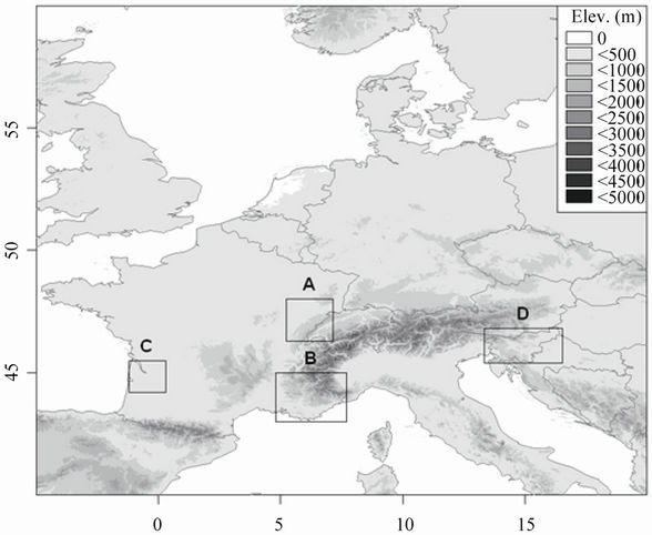
Figure 1. Study areas location with geographical coordinates; A = Franche-Comté, B = PACA, C = Gironde, D = Slovenia.
France) or temperatures recorded at set times (7 am, 2 pm in Slovenia). The data relate to variable numbers of days depending on the areas in question. For Franche-Comté (FC-2006) and PACA daily maxima and minima for the year 2006 are available (Table 1). In Franche-Comté (FC-cold), we have 99 minima for spells of extreme cold (average of the region’s 74 weather stations less than –10˚C) between 1990 and 2007. For Gironde, three years (2003-2005) of records (maxima and minima) are available. For Slovenian temperature measurements at 7 am (close to the daily minimum) and 2 pm (close to the daily maximum) are available for year 2006.
2.3. Topographic Variables
The topographic variables shall be introduced into the regressions as explanatory variables of temperature. They are all taken from a single data source: the 50-m resolution DTM for each of the four study areas. Two types of topographic variable are built: “classic variables” and variables related to landforms.
By “classic” variables, we mean that set of topographic variables that is generally used in most GIS software packages. There are four such variables:
o Altitude [alt] corresponds to the value of pixels read on the DTM. Altitude is not windowed because earlier works have shown that its values vary little from one window to another: altitude is a “non-scalar” [12].
o Slope [slope], and the next four variables are calculated for the eight windows. Slope is the value of inclination from the horizontal (0˚), of the plane of regression obtained from the first-degree polynomial applied to altitudes in each window. Values range in theory from 0 to 90; however, slopes of more than 50˚ are extremely rare.
o Roughness [rough] indicates the unevenness of the relief (it may be zero on a flat or on a perfectly straight incline). It is given by the standard deviation of altitudes relative to the plane of regression.
o Theoretical global radiation [rglob] is calculated for the equinox, as the midday position, between the solstices. It allows for the gradient and aspect of the hillslopes as well as the azimuth and the direction of the Sun. It is calculated hourly and then the 24 values are
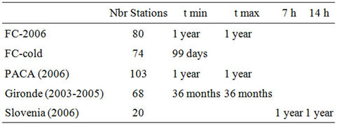
Table 1. Number of weather stations and type of temperature data for the four study areas.
summed to give the daily value. The effect of cast shading is limited to 2 km.
It has been suggested that landforms play an essential part in the spatial structuring of temperature [13,14]. At the end of the night and especially in winter, cold air tends to slide downslope and accumulate in the valley bottoms (catabatic wind) while the hilltops and upper slopes experience milder temperatures. Conversely, in the middle of the day especially if it is warm, warm air is further heated by contact with the ground and tends to rise along hillslopes exposed to the sun (anabatic wind). These thermal effects (slope breezes) influence the temperature well beyond the hillslopes where they are generated. Allowance for such effects has guided the construction of the two topographic variables related to landform: the amplitude of humps [hmp] and of hollows [hllw].
Hump amplitude and hollow amplitude are meant to evaluate the height or depth of a positive or a negative relief relative to a topographic reference point. To calculate these two variables, we proceed in three stages:
o By locating ridgelines and thalwegs and identified in a similar way to with the Peuker-Douglas [15] algorithm. These two linear forms (Figure 2) describe the topographic structure of each study area at different scales.
o By constructing two fictitious topographic surfaces: the “ceiling” passes through all the ridgelines to encompass all of the emerging relief, while the “floor” joins up all the thalwegs (Figure 3). Between the two
Figure 2. Landforms extracted from a DTM for four different windows (from 5 × 5 pixels to 51 × 51 pixels).
surfaces, the distance varies locally with the altitudinal position of the ridgelines relative to the thalwegs. In Figure 3(a), the relief is depicted at high resolution. The main two emergent reliefs are covered by a number of micro-reliefs that give rise to the same number of micro-ridgelines and thalwegs. The ceiling and floor hug the general profile of the topography. The volume enclosed by the two surfaces is small. In Figure 3(b) the relief is shown at lower resolution and so all traces of micro-relief have disappeared, leaving only the major relief. Only the most prominent ridgelines and thalwegs are detected. They are few in number and depict surfaces with a long radius of action, often separated by great distances.
o By calculating the amplitude of forms for any pixel p in the study area. The ridgeline amplitude is obtained by the difference between the altitude of the floor vertically below pixel p and the altitude of pixel p read on the DTM. The depth of the hollows is obtained simply from the difference between the altitude of the ceiling vertically above pixel p and the altitude of pixel p read on the DTM.
Topographic variables are usually estimated from a single DTM pixel or from its nearest four neighbour pixels. The other possibility is to consider larger vicinity through windows of different sizes. Eight concentric circular windows of increasing diameter are calculated for the “classic variables”: 150 m (3 × 3 pixels), 250 m (5 × 5), 550 m (11 × 11), 1050 m (21 × 21), 1750 m (35 × 35), 2500 m (51 × 51), 3750 m (75 × 75) and 5050 m (101 × 101). For technical reasons, the window 3 × 3 is not available for the variables related to landforms (hmp and hllw). This approach allows us to approximate the spatial variation of temperature on different scales, from the smallest (windows 1 or 2 describing the finest topographic variations) to the broadest (windows 7 or 8, which allows for the coarsest tendencies only).
2.4. Method
The Bravais-Pearson correlation coefficients are calculated for the 4481 series of temperature readings (response variables) and the 39 topographic variables (1 + 8 × 3 + 2
Figure 3. Variation of the ceiling and floor on two different scales.
× 7) created in the data base (explanatory variables). The correlation coefficients are subjected to Student’s t tests (at risk a = 5%) to identify which topographic variables significantly accounted for the spatial variability of temperature. The hierarchy of variables is then established on the basis of the frequency with which they are significantly correlated with temperatures.
The results might be skewed by any collinear variables [16]. If two variables have a high common variance, it is likely they will be correlated in the same proportions with the various temperature series. Imagine that steep slopes are all at high altitudes and gentle slopes in the lower lying parts of a given area. In this event, slope and altitude covary to a large extent. If altitude, which is known to influence the spatial variation of temperatures, is frequently correlated with temperature, then the same will be true for slope. Now, if slope influences temperature less than altitude does, the high frequency of slopes as an explanatory variable would be largely due to the collinearity of this variable with altitude. Collinear variables must therefore be reduced to have the clearest possible vision of the variables that best account for the spatial variation of temperatures. There are many sources of collinearity. The example just given (collinearity between altitude and slope) is one. Another source is windowing which induces strong spatial autocorrelation (Table 2). It is inevitable that the values computed for adjacent windows are close since the overlap between windows is high; window 2 (5 × 5 pixels) has 36% of pixels in common with window 1 (3 × 3). However, this collinearity diminishes with increasing difference in window size.
The threshold beyond which the effects induced by collinearity may be detrimental is difficult to determine [17]. Schroeder et al. [18] assert that there are no statistical tests for determining whether or not multi-collinearity. The occurrence of collinearity is evaluated here by the correlation coefficient, which is more intuitive than the “condition index” normally used [19]. In this study, we set it at 0.4 (16% of common variance between pairs of collinear variables).
The main pairings with comparatively high collinearity are a) roughness and slope (r = 0.73), and b) roughness and hump amplitude (0.54) (Table 3). Collinearity is
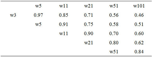
Table 2. Matrix of correlations among the eight windows of the “slope” variable: with PACA as an example.
extremely difficult to handle all around since all of the variables entail some degree of collinearity with the others. After the residuals from these two regressions have replaced the initial values, collinearity in our case study is close to zero (Table 4).
As a result of this processing, most of the other variables are orthogonal or close to it. The collinearity between hump amplitude and roughness has been corrected in part by the “de-correlation” of roughness by altitude: this means that the common variance between these two variables is due in part to the collinearity linking both of them to altitude. The same is true for the collinearity that linked slope to altitude. Let us notice that as to avoid collinearity because of windowing, only the window with the highest r value is selected.
3. Results
Altitude is the variable that significantly explains the spatial variation of temperatures in the greatest number of cases (80%) (Table 5). Statistics clearly show the physical model relating temperature and pressure. Hump amplitude (49%) and hollow amplitude (46%) follow: landforms are involved in nearly half the instances in the spatial variation of temperatures. Behind them lag global radiation
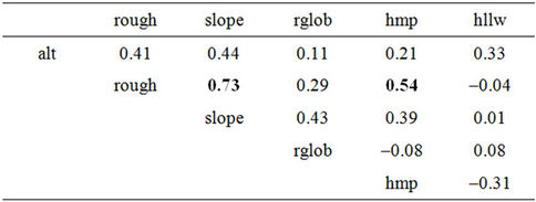
Table 3. Matrix of correlations among the six explanatory variables; with PACA as an example.
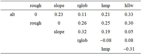
Table 4. Matrix of correlations among the six explanatory variables after de-correlation; with PACA as an example.
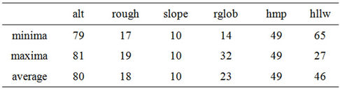
Table 5. Frequency (%) with which the six variables significantly account for the minima and maxima.
(23%) and roughness (18%). Slope is the variable selected least often (10%).
3.1. Variation by Minima and Maxima
The physical processes as highlighted by statistics govern the spatial variation of minima and maxima in very different ways. The largest deviation is for the depth of hollows, which significantly accounts for 65% of the minima and just 27% of the maxima (Table 5). The build-up of cold air in topographic depressions is very marked at the end of the night whereas in the course of the day mechanisms (especially radiation) kick-in to limit its influence. Another important difference between minima and maxima statistics can be observed in the case of global radiation which explains the maxima twice as often as the minima. The other variables (altitude, hump amplitude, roughness and slope) influence the spatial structure of minima and maxima with similar frequencies.
3.2. Variation by Study Area
In Table 6, excess frequencies compared to the average [see Table 5] appear in smaller font and deficit frequencies are in bold print. Temperature variations in PACA, a region of high mountains, depend above all on altitude (significant in 93% of cases) and landforms. FrancheComté fits in with this pattern for the days of extreme cold (FC-cold), where the influence of landforms is even more decisive. Conversely, the spatial structure of temperatures for 2006 (FC-2006) stands apart, except for altitudes, which remain a powerful explanatory variable.
In Slovenia, a mountainous country, altitude while predominant, is more discreet as a variable than in PACA and Franche-Comté. However, the influence of landforms is significant, especially hump amplitude. The role of global radiation in Slovenia is notable, as in FrancheComté. The Gironde, a low-lying area, stands apart. Altitude, as expected, is only significant one day in two whereas the influence of the amplitude of hollows (58%) and the influence of slopes is high.
3.3. Seasonal Variation
Seasonal variations occur in the frequency with which
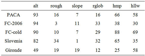
Table 6. Frequency (%) with which the six variables significantly account for the minima in the different study areas (red print = excess compared to the average; blue print = deficit compared to the average).
some topographic variables significantly explain the spatial variations of temperature. We have chosen to present the four variables that most clearly oppose summer to winter.
o Altitude (Figure 4) is less frequently taken as an explanatory variable for spatial variation of minimum and maximum temperatures in winter (74% - 75%) than in spring (78% - 80%) and late summer (85% - 86%). This suggests that in winter heat inversions counter the adiabatic decline in temperature.
o Global radiation (Figure 5) accounts for the spatial variation of maximum temperatures (32%) twice as much as for minimum temperatures (14%). For maxima, its influence rises steadily from January (23%) to June (45%). Then it diminishes until October, from when onwards it levels off at 26%. This variation is consistent with the energy received at the ground surface, which is greater in the afternoons (maxima) than in the mornings (minima). This hypothesis will be discussed later in Section 3.3.
o Landforms influence the spatial variation of minima above all in summertime. Minimum temperatures are influenced on average much more by the amplitude of humps and hollows (56%) than maximum temperatures (38%) are. The frequency with which these two landforms account for the spatial variation of temperature is reversed between the minima and maxima (Figures 6 and 7).
4. Discussion
The results just described should be nuanced by several
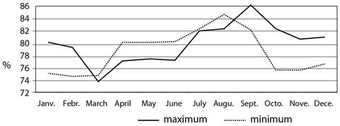
Figure 4. Annual variation of altitude as an explanatory variable for temperature (four study areas).
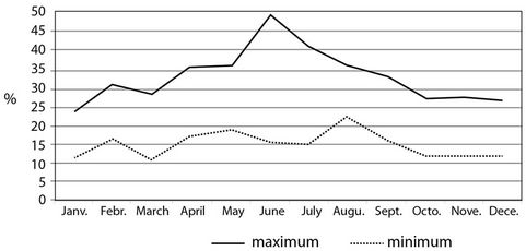
Figure 5. Annual variation of the global radiation as an explanatory variable for temperatures (four study areas).
remarks about windowing, collinearity and the influence of solar radiation on the spatial variation of temperatures.
4.1. Windowing
The windowing system allows to approximate the influence on temperatures of the scales of the topographic variables involved. In some cases, all of the windows significantly explain the variation in temperature. In curve A of Figure 8, the maximum coefficient is in the 21 × 21 window, indicating that it is hollows of a kilometre or so in size that explain most of the spatial variation of minima. In other cases, only one or a few windows exceed the selected level of significance (B). Often none of the windows exceed the threshold (C). But
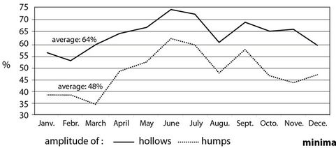
Figure 6. Annual variation in the amplitude of humps and hollows as explanatory variables for minimum temperatures (four study areas).
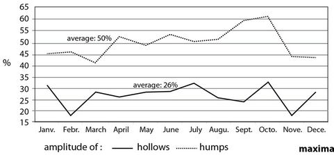
Figure 7. Annual variation in the amplitude of humps and hollows as explanatory variables for maximum temperatures (four study areas).
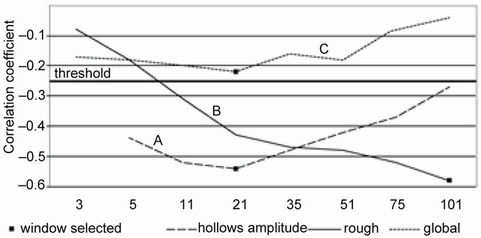
Figure 8. Variation of the correlation coefficient of the amplitude of hollows (A), roughness (B) and global radiation (C) with minimum temperatures for 1 January 2006 in PACA.
regardless of however many windows may have a significant coefficient, the principle of counting occurrences does not allow for double or multiple counting since only the window with the highest r-value is selected. Examination of the windows that are most frequently significant makes it possible to specify which topographic scales are most likely to influence the spatial variation of temperatures. The highest correlation coefficient is obtained by global radiation for the four broadest windows (35 × 35 to 101 × 101) for both minimum (Table 7) and maximum (Table 8) temperatures. It seems that hillslopes have to be extensive if global radiation is to significantly influence temperatures. The heat generated at the ground surface constitutes a micro-airmass large enough to affect the layer of air in the first few metres above the ground only if the receiving hillslope is at least 1750 m in extent. Similar conclusions on the expansion of vegetation cover [12] and extend of slopes [9] had already been made. A similar model affects roughness for maximum temperatures, although no process can be suggested to account for it. With maximum temperatures (Table 8), the amplitude of humps and hollows is most marked in the six broadest windows (from 11 × 11 to 101 × 101). In this case, the only forms that are most rarely selected as explanatory variables for the spatial variation in temperatures are the forms of small extent (less than 250 m). The reverse occurs with the amplitude of hollows for minimum temperatures (Table 7). The most effective cold traps do not seem to be the largest ones.
4.2. Residual Collinearity
One way of measuring the bias introduced by collinearity is to compare the results obtained before and after “de-
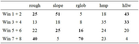
Table 7. Frequency (%) with which the windows two-by-two exhibit significant correlation coefficients; minimum temperatures.
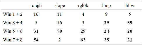
Table 8. Frequency (%) with which the windows two-by-two exhibit significant correlation coefficients; maximum temperatures.
correlation”. Roughness, which displays 16% of common variance with altitude, shall serve as an example. The frequency with which altitude and roughness significantly explain the spatial variation in temperatures is 80% and 43% respectively. After “de-correlation”, roughness explains just 18% of cases (Table 5). The high frequency of “untransformed” roughness as a variable accounting for the spatial variation of temperature is therefore due to its collinearity with altitude; when the collinearity is neutralized, the frequency with which it explains temperatures strongly declines.
4.3. Variation of Global Radiation
Radiation explains significantly more often the temperature variation in summer (than in winter) and the maximum temperatures variation (than the minimum one) (Figure 5). These facts have been explained by the variation in energy received at the ground surface. This interpretation could be contradicted by the observation that radiative differences between north and south facing hillslopes vary much more in winter than in summer: Hufty [20] reports that this difference between two 45 hillslopes exposed one to the north and the other to the south is of 16 MJ/m2/day in winter as against just 6 MJ/m2/day in summer at Carpentras (southern France). It is true that large differences in radiation depending on location is a condition that promotes large temperature differences and therefore a high correlation between these two variables. However, the relation between them is not straightforward and is sometimes difficult to bring out. Accordingly, what is shown in Figure 5 could rather be explained as the response from environments that tend to heat up more with high radiative energy. So the frequency of global radiation as an explanatory variable of the spatial variation of temperature is higher with maximum temperatures and during summer. Global radiation rarely explains the spatial variation of minimum temperatures that ordinarily occur before the sun reaches the station. One should also consider that the theoritical global radiation is a variable that reflects indirectly the terrain aspects, i.e. South and North exposed slopes. Therefore, this variable could be selected as variable explaining the spatial variation of temperature because of temperature differences due to wind effects (shelter/exposure of north and south exposed slopes) depending on the synoptic and the local circulation patterns.
5. Conclusions
Our analysis provides answers to the rank-ordering of variables accounting for the spatial variation of temperatures. First altitude is almost always a significant variable. The only case that does not fit into this model is as expected Gironde because of its moderate topography. The frequency with which altitude is selected is higher when the study area is more mountainous. The amplitude of humps and hollows describes the structure of the topography. We felt their importance and the results we obtained have not disappointed us. It has been shown in many instances that the influence of these landforms on the temperature spatial distribution is often decisive. Their influence is exerted mostly on minimum temperatures, a situation that is strongly influenced by the size of hollows. These two variables are effective above all in PACA and in Franche-Comté during cold spells. As altitude, their introduction in interpolation process is often decisive. Works in progress not yet published show that the estimation errors of temperature and precipitation amount are reduced when they are introduced as explanatory variables. These results more than justify the effort we made to create these variables describing the landforms. Last point, it seems that thalwegs associated with the smallest windows are more explanatory than the thalwegs associated with the broadest windows. It is true that large but shallow valleys may accumulate less cold air that deep but narrow valleys. Also, our future work will focus on calculating the volume of air included in the hollow forms and test if this hypothesis is true or not.
We have voluntarily limited the number of explanatory variables derived from the DTM to six. This has focused attention on a small number of topographic variables accounting for temperature. However, other variables could have been introduced into the analyses, such as the north-south (cosine) and east-west (sine) components of hillslope aspect, distance to the nearest ridgeline, distance to the nearest thalwegs. Statistics show that these additional variables sometimes play a part in the spatial distribution of temperatures. But often it is not easy to derive any physical interpretation from them [9]. Their inclusion in this study would have clouded the results in many instances, although they can be usefully included in interpolation models where the aim is to exploit the maximum number of significant variables.
REFERENCES
- L. Prihodko and S. N. Goward, “Estimation of Air Temperature from Remotely Sensed Surface Observations,” Remote Sensing of Environment, Vol. 60, No. 3, 1997, pp. 335-346. doi:10.1016/S0034-4257(96)00216-7
- K. Czajkowski, S. N. Goward, S. Stadler and A. Walz, “Thermal Remote Sensing of Near Surface Environmental Variables: Application over the Oklahoma Mesonet,” The Professional Geographer, Vol. 52, No. 2, 2000, pp. 345- 357. doi:10.1111/0033-0124.00230
- J. D. Jang, A. A. Viau and F. Anctil, “Neural Network Estimation of Air Temperatures from AVHRR Data,” International Journal of Remote Sensing, Vol. 25, No. 21, 2004, pp. 4541-4554. doi:10.1080/01431160310001657533
- S. Stisen, I. Sandholt, A. Nørgaard, R. Fensholt and L. Eklundh, “Estimation of Diurnal Air Temperature Using MSG SEVIRI Data in West Africa,” Remote Sensing of Environment, Vol. 110, No. 2, 2007, pp. 262-274. doi:10.1016/j.rse.2007.02.025
- K. Zakšek and M. Schroedter-Homscheidt, “Parameterization of Air Temperature in High Temporal and Spatial Resolution from a Combination of the SEVIRI and MODIS Instruments,” ISPRS Journal of Photogrammetry and Remote Sensing, Vol. 64, No. 4, 2009, pp. 414-421. doi:10.1016/j.isprsjprs.2009.02.006
- J.A. Hevesi, J. D. Istok and A. L. Flint, “Precipitation Estimation in Mountainous Terrain Using Multivariate Geosatistics. Part I: Structural Analysis,” Journal of Applied Meteorology, Vol. 31, No. 7, 1992, pp. 661-676.
- C. H. Jarvis and N. Stuart, “A Comparison among Strategies for Interpolating Maximum and Minimum Daily Air Temperatures. Part I: The Selection of “Guiding” Topographic and Land Cover Variables,” Journal of Applied Meteorology, Vol. 40, 2001, pp. 1060-1074.
- D. Joly, L. Nilsen, R. Fury, A. Elvebakk and T. Brossard, “Temperature Interpolation at a Large Scale: Test on a Small Area in Svalbard,” International Journal of Climatology, Vol. 23, No.13, 2003, pp. 1637-1654. doi:10.1002/joc.949
- D. Joly, “Spatial Analysis, Cartography, and Climate. Geographical Information and Climatology,” In: P. Carrega, Ed., Geographical Information and Climatology, ISTE-Wiley, London, 2010, pp. 29-71.
- D. Joly, T. Brossard, H. Cardot, J. Cavailhès, M. Hilal and P. Wavresky, “Types of Climates on Continental France, a Spatial Construction,” Cybergeo European Journal of Geography, Paper 501, 2010. doi:10.4000/cybergeo.23155
- D. Joly, T. Brossard, H. Cardot, J. Cavailhès, M. Hilal and P. Wavresky, “Temperature Interpolation by Local Information; the Example of France,” International Journal of Climatology, Vol. 31, No. 14, 2011, pp. 2141-2153. doi:10.1002/joc.2220
- D. Joly and T. Brossard, “Contribution of Environment Variables to the Temperature Distribution at Different Resolution Levels on the Forefield of the Loven glaciers, Svalbard,” Polar Record, Vol. 43, No. 227, 2007, pp. 353-359.
- R. Geiger, H. Aron and P. Todhunter, “The Climate Near the Ground,” 6th Edition, Rowman & Littlefield Publishers Inc., Lanham, 2003.
- C. D. Whiteman, T. Haiden, B. Pospichal, S. Eisenbach and R. Steinacker, “Minimum Temperatures, Diurnal Temperature Ranges, and Temperature Inversions in Limestone Sinkholes of Different Sizes and Shapes,” Journal of Applied Meteorology, Vol. 43, No. 8, 2004, pp. 1224-1236. doi:10.1175/1520-0450(2004)043<1224:MTDTRA>2.0.CO;2
- T. Peuker and D. H. Douglas, “Detection of Surface-Specific Points by Local Parallel Processing of Discrete TerrainElevation Data,” Computer Graphics and Image Processing, Vol. 4, No. 4, 1975, pp. 375-387. doi:10.1016/0146-664X(75)90005-2
- T. Foucart, “Colinearity and Linear Regressions,” “Colinéarité et Régressions Linéaire, ” Mathématiques et Sciences Humaines (Mathematics and Social Sciences), Vol. 173, No. 1, 2006, pp. 5-25.
- D. Belsey, E. Kuhne and R. Welsch, “Regression Diagnostics: Identifying Influential Data and Sources of Collinearity,” Wiley, New York, 1980. doi:10.1002/0471725153
- L. D. Schroeder, D. L. Sjoquist and P. E. Stephan, “Understanding Regression Analysis,” Sage Publications, Beverly Hills, 1986.
- P. Bressoux, “Modélisation Statistique Appliquée aux Sciences Sociales,” In: Méthodes en Sciences Humaines, de Boeck Université, Bruxelles, 2008.
- A. Hufty, “Introduction à la Climatologie,” de Boeck Université, Bruxelles, 2001, p. 544.