Atmospheric and Climate Sciences
Vol. 2 No. 1 (2012) , Article ID: 17121 , 6 pages DOI:10.4236/acs.2012.21002
Global Warming and the Power-Laws of Ecology
1Physics Institute, University of São Paulo, São Paulo, Brazil
2CEPESq/UniÍtalo, Italy-Brazilian University Center, São Paulo, Brazil
3Laboratory of Cyanobacteria, ESALQ, University of São Paulo, Piracicaba, Brazil
4PROCAM, Interdisciplinary Graduate Program on Environmental Sciences, University of São Paulo, São Paulo, Brazil
5Institute of Oceanography, University of São Paulo, São Paulo, Brazil
6Institute of Biosciences, São Paulo State University, Botucatu, Brazil
7Institute of Biosciences, University of São Paulo, São Paulo, Brazil
Email: arruda@if.usp.br, arruda@usp.br
Received October 20, 2011; revised November 28, 2011; accepted December 16, 2011
Keywords: Global Warming; Species Extinction; Ecology Power-Laws; Species Variability Model
ABSTRACT
A model based on Watson’s power law for the species-area relationship predicts that full global warming, projected up to the year 2050, could provoke the disappearance of roughly one-quarter of existing species. Here, an alternative approach is worked out, based on the combination of two ecology laws: Taylor and Watson’s power laws, where the former relates species variability with their mean abundance. Just how severely global warming would affect not only the number but the diversity of the surviving species is addressed by this approach, while at the same time giving indications for the post-disaster fate of the remaining species (extinction or recovery).
1. Introduction
Many current ecological problems abound such as population viability in conservation biology studies, pest dynamics in agriculture, species diversity and stability, and strategies for environmental monitoring. Addressing these issues requires, in general, a deep understanding of the relationship between population variability (V), its mean abundance (µ) and the area (A) of climatically suitable habitats. Moreover, understanding the factors controlling diversity is high on the agenda for ecologists and conservationists, and different factors evidently operate on different scales [1].
Over the last century the rate of species extinction has been greatly accelerated by various human activities. Rates of extinction are estimated to be 100 to 1000 times higher than pre-human rates [2], and 5 to 20 percent of the species in many groups of organisms have already become extinct [3]. Nowadays, however, temperature is increasingly a prominent factor, which could operate nearly at all scales [4,5]. Besides the already extinct species, concern should be raised for those on the verge of extinction: namely the rare species. In fact, estimating the proportion of rare species in particular habitats is a major issue for ecologists.
Nowadays, the disappearance of species due to habitat destruction seems to be an endless, increasingly aggravated problem one is used to coping with. Additionally, global warming is changing the distribution and abundance of plant and animal species, while there is no evidence that temperatures will stop rising. As yet it is still unclear how great this threat to biodiversity is. In this regard, one modeling study predicts full global warming, projected by the year 2050, which could bring about the disappearance of about one-quarter of existing species [5]. This model relies heavily on Watson’s species-area power law describing how the number of species relates to habitat area.
The rationale of the Thomas model approach is that climate changes induced by escalating higher temperatures are responsible for the reduction of habitat areas, consequently reducing (extinction) the number of species [5]. In fact, analysis of species-area curves has produced a wealth of data, with evidence clearly supporting the obvious rule that if one samples a smaller area, less species will be found [6]. The detailed calculations carried out by Thomas and collaborators, however, did not touch on what would happen to the remaining species on our planet after the apocalyptic year 2050.
Here, it is shown, firstly, that the reduction of habitat areas leads not only to species extinction, but might also lead to changes in the diversity of surviving species. This point is demonstrated by incorporating Watson’s relationship (Equation (2)) into Taylor’s power law (Equation (1)). Finally, by using arguments based on the work by Emerson and Kolm [7], a post-disaster scenario is proposed where the remaining species could oscillate between decay (further extinction) and recovery (speciation), the final fate being decided by the new habitat conditions.
Although not proposing a specific mechanism of extinction, it is advocated here that whatever the mechanism is, the variability of a species would drive its population more or less swiftly toward extinction or recovery after an ecological disaster. In this sense, our approach allows the construction of a “variability phase-space” where, given the species coordinates it would be possible to infer its more probable chances in a post-disaster scenario.
2. The Present Approach-Intertwining Watson’s and Taylor’s Power Laws
2.1. Ecology Power Laws
2.1.1. Taylor’s Power Law
Nearly 25 years ago Taylor and collaborators proposed the so called Taylor’s Power Law, based on the analysis of 156 sets of data of a wide range of species and sampling scales (from ciliates on the surface of a flat-worm to the human population of the United States of America). The model assumed that spatial variance (V) is proportional to a power of the mean population density (m) [8-10],
 (1)
(1)
where α is a proportionality parameter and β is regarded as an “index of aggregation”, taking a characteristic value between 1 and 2 for each species, therefore reflecting the balance between opposing behavioral tendencies to move towards or away from centers of population density. The ubiquity of Taylor’s power-law slopes in the interval 1 < b < 2 is intimately associated with long-range interactions among all the elements of a given system, plus negative interactions among species in a community, as demonstrated by Kilpatrick and Ives [11] using stochastic simulation and analytical models.
2.1.2. Watson’s Power Law
H. C. Watson demonstrated the species-area relationship, which is now a well-established empirical power-law, for Britain’s vascular flora in 1859 and is a relationship describing how the number of species (N) relates to area (A),
 (2)
(2)
where a and b are constants.
From Watson’s Power Law one is able to calculate the amount of species becoming extinct or threatened when the area available to them is reduced by habitat destruction [12,13]. As pointed out elsewhere, the ability of species to reach new climatically suitable areas will be hampered by habitat loss and fragmentation, and their ability to remain in these areas could be affected by new invasive species [5].
2.1.3. Intertwining Watson’s and Taylor’s Power Laws
Consider a given species-i in a habitat with area A. Taylor’s law applied to this particular species is
 (3)
(3)
then,
 (4)
(4)
where Ii is the number of individuals pertaining to the species-i.
In the same vein, from Watson’s law one obtains
 (5)
(5)
which provides a relationship for the area, that is,
 (6)
(6)
By substituting Equation (6) in Equation (4) and then in Equation (3) we obtain
 (7)
(7)
where k = αi·aβ/b. It should be emphasized that this new expression (Equation (7)) relates the variability of species-i with both its population (Ii) and the total number of species (N) present in the habitat area A .
The total population of the community with N species is I = Σ Ii, where i = 1, 2, 3… N.
If, by any reason, the total number of species living in a habitat area A is reduced by a factor r (0 < r < 1) from its initial value N to a final value
 (8)
(8)
while the population Ii of species-i changes by a factor si (si > 1, or si < 1) to
 (9)
(9)
the corresponding variability would change from Vi to Vi*. From Equation (7) one straightforwardly obtains
 (10)
(10)
by assuming b = 0.25 [5] we get
 (11)
(11)
However, the actual value for b would be determined from some assumptions on extinction mechanisms and the remaining habitat areas.
The condition to obtain no change in the variability, that is, Vi* = Vi, is si = r4. In Figure 1, curve (1), a plot of the function si(r) = r4 is shown, which here is named iso-variability curve, dividing the coordinate plane (here referred to as the variability phase-space) in two halfplanes corresponding to Vi*/Vi > 1 and Vi*/Vi < 1.
2.2. Minimum Population Size
The concept of “minimum population size” (m) was introduced by Preston [14] in terms of what he called “logarithmically Gaussian universe”, where its geometrical objects are “lognormal curves”. Two of these were the Species and Individual Curves, both presenting the same variable as abscissa: the total number of individuals per species interval. From a numerically transparent analysis of the modes and logarithmic standard deviation of these two curves, one obtained by linearization procedures (least-squares fitting)
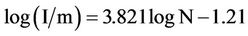 (12)
(12)
(see Equation (12) in [14])
where I is the total number of individuals in the whole ensemble, and m is the minimum number of individuals that may be assumed necessary to keep a species in existence.
Applying the inverse logarithm operation in Equation (12) we obtain
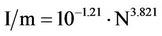 (13)
(13)
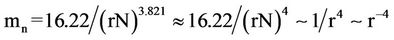
Our alternative interpretation for this result, far more adequate for the present study, is to consider the inverse of I/m, that is,
 (14)
(14)
The ratio m/I (mn) is a “normalized minimum population size”, expressing how much each individual contributes to the total m. Also, it allows for the appraisal of m independently of the population size of all participating species (N). It is, in fact, a “collective” parameter, i.e., it depends on “totals” (I and N) and not on the peculiarities of a single species. Because of this, Preston succeeded in deriving the Watson power law from the approximation that individuals are distributed uniformly over wide areas (further details in [14]).
One may express Equation (14) as function of r (see Equation (8)) by simply redefining mn as
 (15)
(15)
where r runs from 1 to zero. This function defines the curve mn(r) = r–4, dividing the phase-space in two other semi-planes, where in one of them species cannot exist, the “extinction zone” (shaded band in Figure 1).
3. Phase-Space Analysis
Curve-1 in Figure 1 is the iso-variability curve (see Equation (11)), si(r) = r4. The factor r (0 < r < 1), expressing the reduction of the total number of species living in
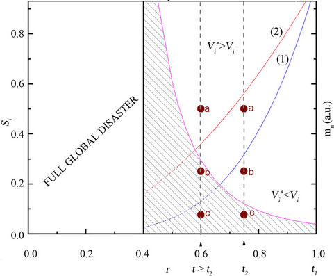
Figure 1. The continuous curves (1) and (2) represent the function si/rb = 1 for b = 4 and b > 4, respectively. According to Equation 11, these isovariability curves split the phasespace into two regions, corresponding to increasing and decreasing variabilities, Vi* > Vi and Vi* < Vi , respectively. The shaded band (extinction zone) is defined by the function mn(r) ~ r–4 (Equation 15) – right-handed scale (arbitrary unities). The points a, b and c represent examples of post-disaster species. In the abscissa axis, t1 (pointing to r = 1) and t2 (pointing to r = 0.75) correspond to the present-time and the year 2050, respectively (see text for details).
a given habitat area, may be related to time (t). In this case, t1 in the abscissa axis (pointing to r = 1) corresponds to present-time, thus implying that variation of species number and population is inventoried from now on (si = r = 1).
In order to illustrate the use of the variability phasespace, the scenario predicted for the year 2050 (t2 in the abscissa—Figure 1), i.e., extinction of one quarter of the existing species (r = 0.75) is assumed [5]. With the abscissa fixed e.g. at r = 0.75, all (r, si) points lie in a straight line parallel to the ordinates axis. The determination of the relative position of each (r, si) point depends on the post-disaster inventory of the actual populations, that is, Ii* at t = t2 (si = Ii*/Ii).
Therefore, the analysis based on the study approach starts only after the location of (r, si) in the phase-space. In Figure 1 possible locations (labeled a, b and c) are exemplified Additionally, it is assumed that the fate of a species (stability, recovery or extinction) is strongly dependent on the semi-plane where it will be located, except for those doomed species falling in the extinction zone (location-c in Figure 1). Those rare species with population sizes near mn have a nontrivial regime, because such species grow differentially faster than common species and, therefore, move up and out of the rarest abundance categories owing to their rare-species advantage [15].
3.1. The Year After
What matters for a given post-disaster surviving species-i is 1) the fraction of its remaining population size, si, at t = t2 , since this determines the position in the phase-space (Vi* > Vi or Vi* < Vi semi-planes), and 2) the ability to increase its population size in order to move up to the region of higher variability. Since si = r4 = 0.754 = 0.32, the remaining species population in the Vi* > Vi (Vi* < Vi) semi-plane are higher (smaller) than 32% of the population at t = t1. Then (Figure 1),
1-species location-a (Vi* > Vi )
Species in this region have relatively more chances of overcoming most of their difficulties. These are species which have maintained more than 40% - 50% of their original population, and that will dispute the available habitat area. They display more stability because Vi* > Vi, and could contribute to the enhancement of speciation.
2-species location-b (Vi* < Vi )
A regime of decreasing diversification (Vi*/Vi < 1) would constrain and/or prevent recovery of the species number plus an associated smaller rate of diversification (discussed below). This is a rather uncertain and unstable situation because of the proximity of the extinction zone (shaded band in Figure 1).
Thus, assuming that after a predicted global warming temperature stabilizes within a relatively short period of time, habitat areas are no longer appreciably reduced (keeping the remaining number of species fixed for some time). Therefore, species in the Vi*/Vi > 1 region would be entitled to bounce back and forth, alternating recovery and decay of their variability. Here this ecokinetics is called recover/decay loop. The argument supporting this possibility is the following:
As less (more) species come into play, competition would assume a smaller (greater) role, with population size facing a decreased (increased) probability of competitive exclusion and predation [6]. Since the remaining and reduced habitat area is not appreciably changing, this would maintain species oscillating in the recover/decay loop; pictorially shown in Figure 2 as a self-explained block-scheme.
3.2. Many Years After
There is reasonable consensus that even if one stopped emitting heat-trapping gases immediately, the climate would not stabilize for many decades because the gases already released into the atmosphere will stay there for years or even centuries to come. Thus, although warming could be lower, or increase at a slower rate than predicted, if emissions are reduced significantly, global temperatures will be unable to quickly return to today’s averages.
With such a possibility in mind, it would be instructive to speculate on how the global scenario would be if temperature kept rising a few decades after 2050. Thus, with
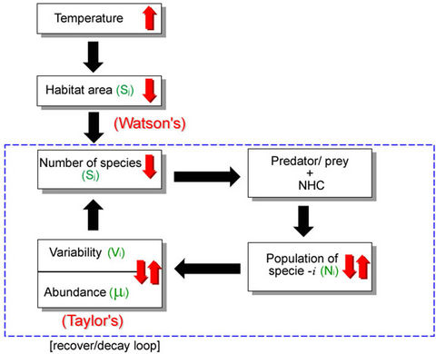
Figure 2. Schematic block diagram showing the sequence of events in a self-explaining way, starting from an increase in temperature (arrow up in the corresponding block). The decay/recover loop represents a hypothetical situation where the surviving species are altering their speciation rate (details in the text). NHC stands for new habitat conditions.
additional loss of habitat and species, the abscissa in the phase-space would be displaced from r = 0.75 (at t2) to a lower value, say r = 0.6 (at t > t2), as illustrated in Figure 1. Also, the increasing fragmentation of habitat moves the isovariability curve upwards toward higher population sizes (curve-2 in Figure 1), shrinking even more the Vi*/Vi > 1 region, therefore making recovery more difficult and uncertain. The faster and continuously the Earth warms, the greater the chances are for irreversible climate changes, up to the point where applicability of current ecology laws is no longer valid.
4. Final Remarks
Emerson and Kolm in their “Species diversity can drive speciation” candidly pointed out that, “The answer to questions such as why there are so many species in the tropics might in part be because there are so many species in the tropics” [7].
But, finally, what are the consequences for species encountering living conditions where diversity is decreasing? The two ecology power laws cannot provide a direct answer to this question. However, Emerson and Kolm analyzing data for plants and arthropods of the volcanic archipelagos of the Canary and Hawaiian Islands did find a positive relationship between species diversity and rate of diversification. They showed, additionally, that even after controlling several important physical features of islands, diversification is strongly related to species number.
All this indicates, therefore, that a regime of decreasing diversification (Vi*/Vi < 1) would prevent recovery of the species number plus an associated smaller rate of diversification. In order to appraise additional, longer term drawbacks associated with decreasing diversification, it is to be recalled that only increasing species diversity can lead to greater community structural complexity, which has been suggested as a possible evolutionary force driving speciation [16].
It becomes increasingly clear that only with diversity would it be possible to achieve effective conservation of both resilience and interconnectivity. Theoretical studies suggest that the risk of secondary extinctions, for example, decreases with increasing biodiversity (measured as average number of species per functional group) in model food webs [17-19]. There are also field experiments suggesting that increased number of species in the different functional groups enhances the functional reliability of the community [20,21].
Once it is agreed that an ecological community behaves as a network of interconnected elements, can one access the most profound aspects regulating its functioning and, consequently, attain new insights for the conception of new models, while improving on existing ones. Until now, for instance, there has been no analytical derivation of the expected equilibrium distribution of relative species abundance in local communities, and fits to the theory have required simulations [22].
In this sense, the approach presented here could contribute to supporting and providing clues for the general understanding of patterns of species richness and community composition following a severe disaster scenario such as global warming, whilst calling into question the validity of models that do not incorporate the crucial issue of species diversity.
5. Acknowledgements
This study was supported by grants from FAPESP, CNEN and CNPq, Brazilian funding agencies for the promotion of science.
REFERENCES
- A. M. Kilpatrick and A. R. Ives, “Species Interactions Can Explain Taylor’s Power Law for Ecological Time Series,” Nature, Vol. 422, No. 6927, 2003, pp. 65-68. doi:10.1038/nature01471
- S. L. Pimm, G. J. Russel, J. L. Gitleman and T. M. Brooks, “The Future of Biodiversity,” Science, Vol. 269, No. 5222, 1995, pp. 347-350. doi:10.1126/science.269.5222.347
- J. H. Lawton and R. M. May, “Extinction Rates,” Oxford University Press, Oxford, 1995.
- J. A. Pounds and R. Puschendorf, “Clouded Futures,” Nature, Vol. 427, 2004, pp. 107-109. doi:10.1038/427107a
- C. D. Thomas, “Extinction Risk from Climate Change,” Nature, Vol. 427, No. 8, 2004, pp. 145-148. doi:10.1038/nature02121
- M. L. Rosenzweig, “Species Diversity in Time and Space,” Cambridge University Press, Cambridge, 1995. doi:10.1017/CBO9780511623387
- B. C. Emerson and N. Kolm, “Species Diversity Can Drive Speciation,” Nature, Vol. 434, No. 7036, 2005, pp. 1015-1017. doi:10.1038/nature03450
- L. R. Taylor, I. P. Woiwod and J. N. Perry, “The Density Dependence of Spatial Behavior and the Rarity of Randomness,” Journal of Animal Ecology, Vol. 47, 1978, pp. 383-406. doi:10.2307/3790
- L. R. Taylor and I. P. Woiwod, “Temporal Stability as a Density-Dependent Species Characteristic,” Journal of Animal Ecology, Vol. 49, No. 1, 1980, pp. 209-224. doi:10.2307/4285
- L. R. Taylor and I. P. Woiwod, “Comparative Synoptic Dynamics: Relationships between Interspecific and Intraspecific Spatial and Temporal Variance-Mean Population Parameters,” Journal of Animal Ecology, Vol. 51, No. 3, 1982, pp. 879-906. doi:10.2307/4012
- A. M. Kilpatrick and A. R. Ives, “Species Interactions Can Explain Taylor’s Power Law for Ecological Time Series,” Nature, Vol. 422, No. 6927, 2003, pp. 65-68. doi:10.1038/nature01471
- T. M. Brooks, S. L. Pimm and N. J. Collar, “Deforestation Predicts the Number of Threatened Birds in Insular Southeast Asia,” Conservation Biology, Vol. 11, No. 2, 1997, pp. 382-394. doi:10.1046/j.1523-1739.1997.95493.x
- T. M. Brooks, S. L. Pimm and J. O. Oyugi, “Time Lag between Deforestation and Bird Extinction in Tropical Forest Fragments,” Conservation Biology, Vol. 13, No. 5, 1999, pp. 1140-1150. doi:10.1046/j.1523-1739.1999.98341.x
- F. W. Preston, “The Canonical Distribution of Commonness and Rarity: Part I,” Ecology, Vol. 43, No. 2, 1962, pp. 185-215. doi:10.2307/1931976
- J. Chave, H. C. Muller-Landau and S. A. Levin, “Comparing Classical Community Models: Theoretical Consequences for Patterns of Diversity,” American Naturalist, Vol. 159, No. 1, 2002, pp. 1-23. doi:10.1086/324112
- M. Tokeshi, “Coexistence: Ecological and Evolutionary Perspectives,” Blackwell Science, Oxford, 1999.
- C. Borrvall, R. Ebenman and T. Jonsson, “Biodiversity Lessens Risk of Cascading Extinction in Model Food Webs,” Ecology Letters, Vol. 3, No. 2, 2000, pp. 131- 136. doi:10.1046/j.1461-0248.2000.00130.x
- S. L. Pimm, “Complexity and Stability: Another Look at MacArthur’s Original Hypothesis,” Oikos, Vol. 33, No. 3, 1979, pp. 351-357. doi:10.2307/3544322
- S. L. Pimm, “Food Web Design and the Effect of Species Deletion,” Oikos, Vol. 35, 1980, pp. 139-149. doi:10.2307/3544422
- D. Tilman, D. Wedin and J. Knops, “Productivity and Sustainability Influenced by Biodiversity in Grassland Ecosystems,” Nature, Vol. 379, No. 6567, 1996, pp. 718- 720. doi:10.1038/379718a0
- D. Tilman, J. Knops, D. Wedin, P. Reich, M. Ritchie and E. Siemann, “The Influence of Functional Diversity and Composition on Ecosystems Processes,” Science, Vol. 277, No. 5330, 1997, pp. 1300-1302. doi:10.1126/science.277.5330.1300
- S. P. Hubbell, “The Unified Neutral Theory of Biodiversity and Biogeography,” Princeton University Press, Princeton, 2001.