International Journal of Astronomy and Astrophysics
Vol. 3 No. 2 (2013) , Article ID: 32348 , 6 pages DOI:10.4236/ijaa.2013.32009
The Evolution QSOs—The Optical Luminosity Function
1Department of Physics, Pettigrew College, Ukhrul, India
2Department of Physics, Manipur University, Canchipur, India
Email: ablu.irom@gmail.com, yugindro361@gmail.com
Copyright © 2013 Irom Ablu Meitei, K. Yugindro Singh. This is an open access article distributed under the Creative Commons Attribution License, which permits unrestricted use, distribution, and reproduction in any medium, provided the original work is properly cited.
Received March 4, 2013; revised April 2, 2013; accepted April 10, 2013
Keywords: Galaxies; Active
ABSTRACT
Using the data of the 2 Degree Field (2dF) QSO Redshift Survey (2QZ) and the associated 6 Degree Field (6dF) QSO Redshift Survey (6QZ) of the Anglo-Australian Telescope, a study of the Optical Luminosity Function of Quasi Stellar Objects (QSOs) has been made to understand the evolutionary scenario of QSOs. Different models for the QSO evolution are studied. The two-power law model of the optical luminosity function with second order polynomial evolution is found to fit best the observed QSO optical luminosity function. We have also determined an improved evolutionary model which fits better than the second order polynomial evolution model. The best fit parameters for the observed optical luminosity function have been determined using the Levenberg-Marquardt algorithm of non-linear least square fit for a flat universe i.e., ΩΛ + Ωm = 1 and Ho = 70 km·s–1·Mpc–1. The observed slope of the log N − m curve i.e., 1.10 ± 0.01 reveals that there were more QSOs at larger distances (or look back times) than there are locally which, in turn, indicates that the QSOs are evolving. The observed value of
1. Introduction
The Quasi Stellar Objects (QSOs) constitute an evolving population. Their cosmological evolution was established by Schmidt (1968) [1] by applying the “V/Vmax” test. If the evolution of an ensemble of the QSOs can be satisfactorily described, some clues as to the evolution of the individual sources may be apparent and these may lead to a better understanding of the physics of the QSO phenomenon [2]. Therefore, it is expected that the QSO evolution would throw light on the energy generation mechanism in the Active Galactic Nuclei (AGNs). Such an evolutionary scenario would also reveal information on the relationship between the QSOs and the normal galaxies. The QSOs represent an important phase of galactic evolution. Some papers e.g. [3-6] proposed joint evolutionary models of galaxies and QSOs in which mergers between gas rich galaxies drive nuclear inflow of gas fueling the growth of supermassive black holes until feedback (e.g. galactic wind) energy from black hole growth expels the surrounding gas rendering the QSO as a briefly visible bright optical source. Lapi et al. (2008) [7] proposed a model in which the QSO activity marked a transition between an earlier phase of violent and heavily dust shrouded starburst activity which promotes rapid black hole growth, and a later phase of almost passive evolution.
The luminosity function provides a basis for determining the amount of matter in different forms in the universe [8]. The optical luminosity function of the QSOs and its evolution with redshift provides fundamental information on the demographics of the overall population of the AGNs. It is a useful instrument to quantify the activity statistics of the AGNs [9]. The optical luminosity function of the QSOs and the Seyfert nuclei join smoothly. The shape, normalization and evolution of the luminosity function are among the most basic descriptions of the QSO population and hence of the AGNs in general [10]. The optical luminosity function of QSOs as a function of redshift provides essential constraints on how the population characteristics of the QSOs have changed with time (Koo & Kron, 1988) [2] and also provides constraints on the physical models of the QSOs [11]. Further, it may provide information on the models of structure formation in the early universe [12].
Croom et al. 2009 [13] observed flattening of the luminosity function towards faint absolute magnitudes in their study of the QSO luminosity function of the 2dFSDSS LRG and QSO (2SLAQ) survey. Clear evidence of downsizing was observed i.e. the number density of faint QSOs peaks at lower redshift than do the bright QSOs. The bright end of the QSO luminosity function tells us about the intrinsic properties of the QSO population during the time when the black holes are increasing in mass rapidly whereas the faint end of the QSO luminosity function tells us about the length of time QSOs spend at relatively low accretion rates [14]. Fontanot et al. 2007 [14] computed the QSO contribution to the UV background at high redshift using the method proposed by Barger et al. 2003 [15] and confirmed that the QSO contribution to the UV background was insufficient for ionizing the intergalactic medium at these redshifts.
A brief description of the 2QZ and the 6QZ data is given in Section 2. Simple tests for the evolution of the QSOs are described in Section 3 and the study of the optical luminosity function in Section 4.
2. The Data
The 2-degree Field (2dF) QSO Redshift Survey (2QZ) and the associated 6-degree Field (6dF) QSO Redshift Survey (6QZ) catalogues are used for the study of QSOs and their evolution. These surveys provide more than 23,500 QSOs in a single homogeneous survey covering almost five magnitudes in the bJ band (16 < bJ < 20.85).
The QSO candidates for the 2QZ and 6QZ surveys are selected based on the broadband ubJr colours for the automated plate measurement (APM) of UK Schmidt Telescope (UKST) photographic plates. Details are given in [16]. The survey region comprises of 30 UKST fields arranged in two 75˚ × 5˚ declination strips, one passing across the South Galactic Cap (SGP) centred on δ = –30˚ (SGP) strip and the other across the Northern Galactic Cap (NGP) centred on δ = 0˚ (referred to as the equatorial strip, also known as the NGP strip) The SGP strip extends from α = 21h 40 to α = 3h 15 and the equatorial strip from α = 9h 50 to α = 14h 50 (in B1950 coordinate system). The total survey area is 721.6 deg2, when allowance is made for regions of sky exercised around bright stars.
The QSO candidates were selected based on fulfilling at least one of the following colour criteria: u – bJ ≤ – 0.36; u – bJ ≤ 0.12 – 0.8(bJ – r); bJ – r < 0.05. The u – bJ limit was tightened to u – bJ ≤ –0.50 for the 6QZ sample (bJ ≤ 18.25) so as to reduce the high fraction of contamination by galactic stars (for details see [17]).
3. Simple Tests for Evolution of QSOs
3.1. The Log N – m Test
We can test whether the space density of a population of a particular class of objects is constant or not by plotting the logarithm of the cumulative distribution, N as a function of the apparent magnitude, m and measuring the slope. A slope dlogN(m)/dm > 0.6 indicates that the space density increases with distance [18,19]. The plot of log N versus m plot for the 2QZ and 6QZ QSOs is shown in Figure 1. The apparent magnitude, m is taken in the bJ band. The slope of the most luminous QSOs is observed as 1.10 ± 0.01 which indicates that there were more QSOs at larger distances ( or look back times) than there are locally, i.e. there were more QSOs in the past, indicating a strong evolution of the QSOs.
3.2. The Luminosity—Volume Test (V/Vmax Test)
The luminosity-volume test was devised by M. Schmidt [1] to test for the evolution of a population of objects. The test, also known as the V/Vmax test was first used by Schmidt to study the space distribution of a complete sample of radio quasars from the 3CR catalogue. A uniform distribution of objects is characterized by the
4. The QSO Optical Luminosity Function
A binned estimate of the differential optical luminosity function has been determined using the 1/V estimator devised by Page & Carrera [20]. The QSOs in the redshift range z = 0.3 to z = 2.3 are divided into eight equal intervals 0.3 ≤ z ≤ 0.55, 0.55 ≤ z ≤ 0.80, 0.80 ≤ z ≤ 1.05,
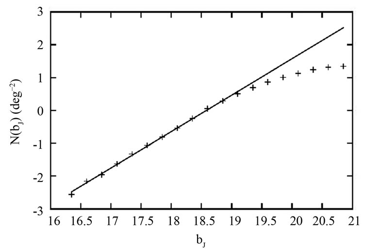
Figure 1. Log N – m plot for the 2QZ and 6QZ QSOs. Here N is the cumulative number distribution of the QSOs and m, the apparent magnitude taken in the bJ band. The line shown is best fit line for the luminous QSOs.
1.05 ≤ z ≤ 1.30, 1.30 ≤ z ≤ 1.55, 1.55 ≤ z ≤ 1.80, 1.80 ≤ z ≤ 2.05 and 2.05 ≤ z ≤ 2.30. Each redshift interval is binned into bins in absolute magnitude with bin width, .
.
For ΩΛ = 0.7 universe, the binned luminosity function is shown in Figure 2. We have used the Hubble constant, Ho = 70 km·s–1·Mpc–1. The downturn at the faint end of the luminosity function is due to incompleteness of the corresponding bins [21]. These incomplete bins are not included in our study of the QSO luminosity function. Similarly, for ΩΛ = 0.0, 0.3, 0.5 and 0.9 the incomplete bins have been ignored. We have assumed a flat Universe, i.e. ΩΛ + Ωm = 1. The routine mrqmin given in [22] based on the Levenberg—Marquardt method and the associated routines are used to fit the observed optical luminosity function to various models. Since the bright end of the luminosity function is steeper than the faint end despite the absence of a sharp break, a two-power-law function in the luminosity,  is used to model the optical luminosity function,
  [9,17-19,23,24]:
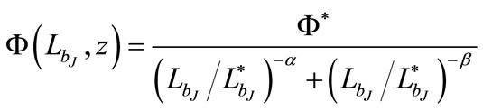 (1)
(1)
In terms of magnitude,
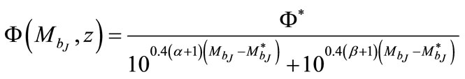 (2)
(2)
The evolution of the luminosity function is given by the redshift dependence of the characteristic or break luminosity,  or break magnitude,
 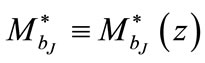 . Different models of the luminosity evolution are studied to determine the best fit parameters for different cosmologies ΩΛ = 0.0, 0.3, 0.5, 0.7 and 0.9.
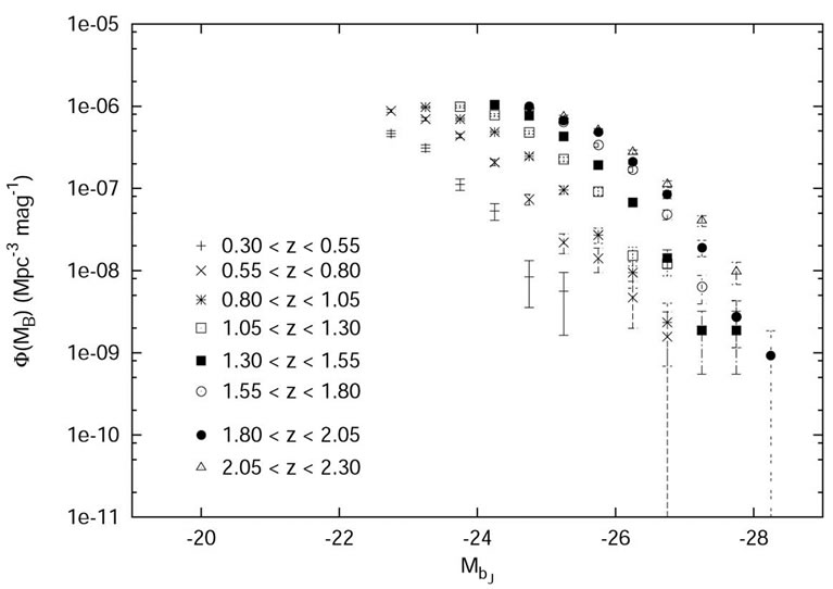
Figure 2. Binned estimate of the optical luminosity function,  as a function of the absolute magnitude,
  in the bJ band for the 2QZ/6QZ QSOs in the redshift range 0.3 ≤ z ≤ 2.3 for a flat Universe with cosmological constant, ΩΛ = 0.7 and Hubble constant, Ho = 70 km·s–1·Mpc–1.
These models include
1) , or equivalently,
  , the power law evolution with redshift, z;
2) , or equivalently,
  , the second-order polynomial evolution model;
3) , or equivalently,
  , the exponential evolution with look-back time, τ.
These three models have already been used in several well-known papers e.g. [9,17,23,24].
To find an alternative model the exponent “2” of z in the second order polynomial evolution model is replaced by a parameter which is varied to give a value that minimizes the χ2. It is observed that the minimum of χ2 is obtained when the parameter is 1.47. Thus, another luminosity evolution model given by
 , or equivalently,

is determined. The luminosity functions and the predictions of the best fitting luminosity evolution model  and the best fit second order polynomial evolution model are shown in Figures 3 and 4 respectively. The best-fitting parameters, the χ2 values, the degrees of freedom ν, P(χ2) and the cosmological constant ΩΛ for different evolution models are given in Table 1.
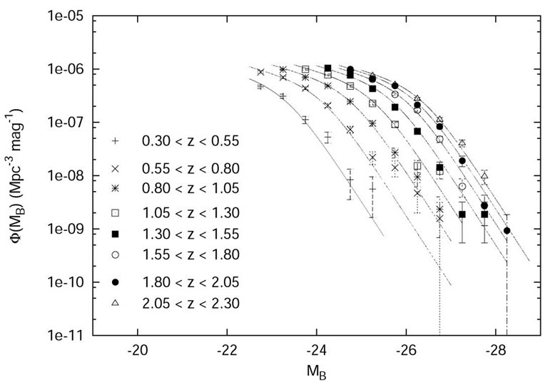
Figure 3. Binned estimate of the optical luminosity function, 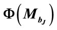 as a function of the absolute magnitude,
  in the bJ band for the 2QZ/6QZ QSOs in the redshift range 0.3 ≤ z ≤ 2.3 for a flat Universe with cosmological constant, ΩΛ = 0.7 and Hubble constant, Ho = 70 km·s–1·Mpc–1. The dotted lines denote the predictions of the best fitting twopower law with the evolution model k1z + k2z1.47.
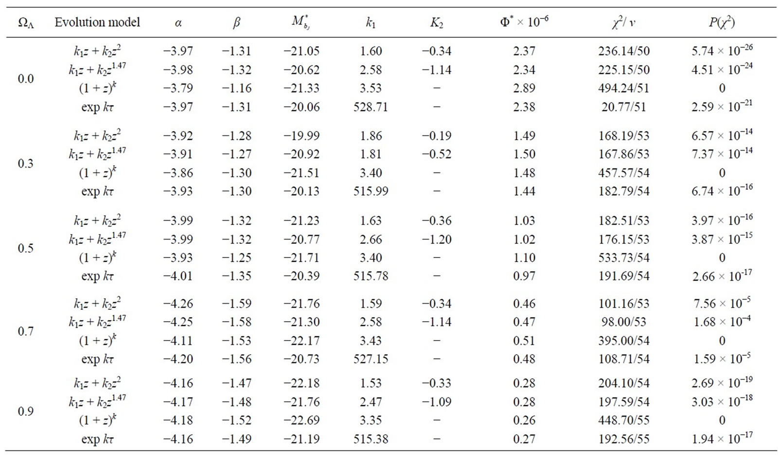
Table 1. The best fitting optical luminosity function model parameter for the QSOs with redshift 0.3 ≤ z ≤ 2.3 and  for a flat universe i.e. ΩΛ + Ωm = 1 and Ho = 70 km·s–1·Mpc–1. The cosmological constant, ΩΛ, the evolution models, the χ2, degrees of freedom ν and P(χ2) are also listed.
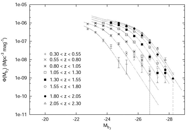
Figure 4. Binned estimate of the optical luminosity function,  as a function of the absolute magnitude,
  in the bJ band for the 2QZ/6QZ QSOs in the redshift range 0.3 ≤ z ≤ 2.3 for a flat Universe with cosmological constant, ΩΛ = 0.7 and Hubble constant, Ho = 70 km·s–1·Mpc–1. The dotted lines denote the predictions of the best fitting two-power law with the second order polynomial evolution model.
The statistical errors on the individual parameters determined using Monte Carlo simulation are σ(Φ*) = 0.04 × 10⁻⁷ Mpc–3·mag–1; ; σ(k1) = 0.06; σ(k2) = 0.06; σ(α) = 0.01; σ(β) = 0.02 for the evolution model
  .
.
The χ2 values for the power law evolution with redshift  are exceedingly high and the P(χ2) values are very small. And for the exponential evolution model convergence of the χ2 is not achieved. However, for the sake of completeness the estimated parameters are listed.
From Table 1, it is observed that luminosity evolution of the QSO optical luminosity function is best described by the new model 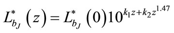 with P(χ2) = 1.68 × 10⁻⁴. And the second order polynomial evolution model is also acceptable with P(χ2) = 7.56 × 10⁻⁵.
The value of k1 is larger than the values reported in the earlier papers e.g. [9,13,17,23,24]. The best fit bright end slope of the luminosity function is steeper as compared to the earlier results. The inclusion of QSOs with lower spectroscopic completeness, a large fraction of which goes to the fainter magnitudes might have contributed to the steepening of the luminosity function. However, the slope of the faint end of the luminosity function agrees well with the earlier results. The values of the constant k for the model of exponential evolution with look-back time are found to be exceedingly high compared to the values reported in the above papers. The failure of the convergence of the χ2 to less than or equal to 0.01, which we have used as the convergence criterion might be responsible for the large value of k. The form of the look-back time coupled with the two-power-law form of the luminosity function might have led to the nonconvergence.
The number of the observed, Nobs and predicted, Npred QSOs for the best-fitting luminosity evolution model k1z + k2z1.47 are given in Table 2.
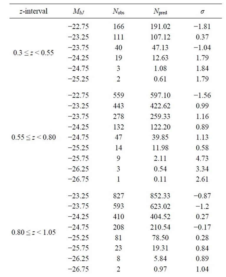
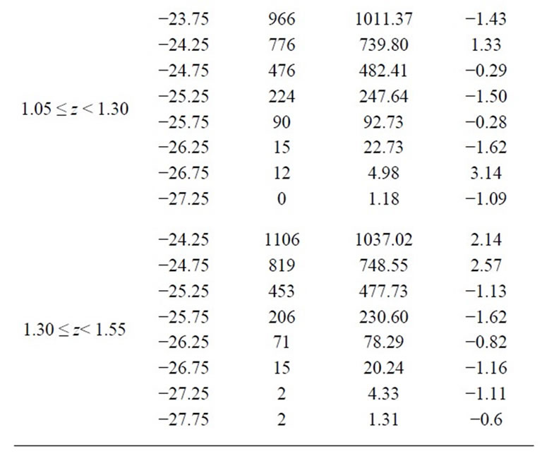
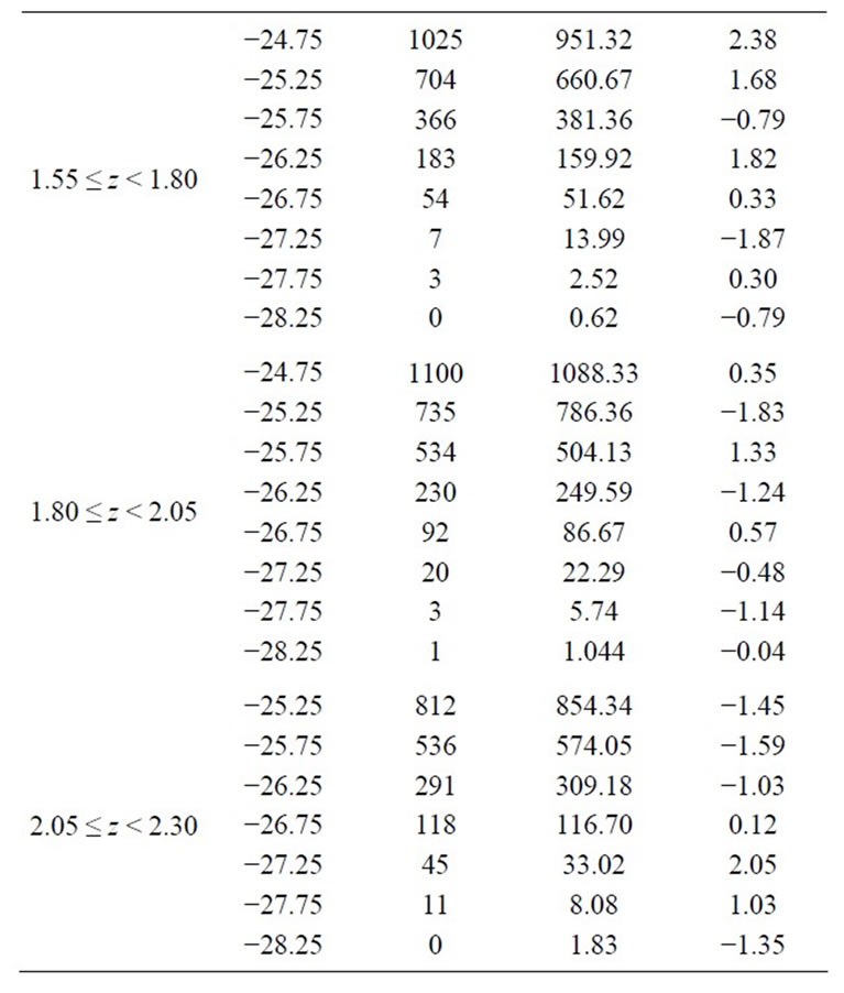
Table 2. The number of the observed, Nobs and predicted, Npred QSOs for the best-fitting luminosity evolution model k1z + k2z1.47 using ; 0.3 ≤ z ≤ 2.30 and ΩΛ = 0.7, Ho = 70 km·s−1·Mpc−1 for a flat universe i.e. ΩΛ + Ωm = 1.
5. Conclusion
A study of the evolutionary scenario of the 2QZ and the associated 6QZ QSOs is carried out. A modest attempt is made to parameterize the QSO evolution using the optical luminosity function. An improved evolutionary model in the framework of the two-power-law model of the optical luminosity function which fits the observed QSO optical luminosity function, is determined. The best fit parameters for the QSO optical luminosity function are also determined. A complete understanding of the optical luminosity function would reveal information on the AGN phenomena, the relation between the normal galaxies and the AGNs and also about the structure formation in the early universe. Of the five values of the cosmological constant, ΩΛ, the χ2 value is found to be minimum for ΩΛ = 0.7 which agrees with the most widely accepted value. This shows that the study of the optical luminosity function might provide a tool for estimation of the value of the cosmological constant. It is hoped that information contained in the QSO population in the form of the optical luminosity function would reveal the nature of the QSO energy source and help to constrain the values of some of the cosmological parameters.
6. Acknowledgements
The 2dF QSO Redshift Survey (2QZ) was compiled by the 2QZ survey team from observations made with the 2- degree Field on the Anglo-Australian Telescope. The authors are thankful to the entire 2QZ/6QZ team.
REFERENCES
- M. Schmidt, “Space Distribution and Luminosity Functions of Quasi-Stellar Radio Sources,” The Astrophysical Journal, Vol. 151, No. 2, 1968, pp. 393-409. doi:10.1086/149446
- D. C. Koo and R. G. Kron, “Spectroscopic Survey of QSOs to B = 22.5: The Luminosity Function,” The Astrophysical Journal, Vol. 325, No. 1, 1988, pp. 92-102. doi:10.1086/165984
- P. F. Hopkins, et al., “Black Holes in Galaxy Mergers: Evolution of Quasars,” The Astrophysical Journal, Vol. 630, No. 2, 2005, pp. 705-715. doi:10.1086/432438
- P. F. Hopkins, et al., “Luminosity-Dependent Quasar Lifetimes: A New Interpretation of the Quasar Luminosity Function,” The Astrophysical Journal, Vol. 630, No. 2, 2005, pp. 716-720. doi:10.1086/432463
- P. F. Hopkins, et al., “A Unified, Merger-Driven Model of the Origin of Starbursts, Quasars, the Cosmic X-Ray Background, Supermassive Black Holes, and Galaxy Spheroids,” The Astrophysical Journal Supplement Series, Vol. 163, No. 1, 2006, pp. 1-49. doi:10.1086/499298
- P. Monaco and F. Fontanot, “Feedback from Quasar in Star-forming Galaxies and the Triggering of Massive Galactic Winds,” Monthly Notices of the Royal Astronomical Society, Vol. 359, No. 1, 2005, pp. 283-294. doi:10.1111/j.1365-2966.2005.08884.x
- A. Lapi, et al., “Quasar Luminosity Functions from Joint Evolution of Black Holes and Host Galaxies,” The Astrophysical Journal, Vol. 650, No. 1, 2006, pp. 42-56. doi:10.1086/507122
- P. Osmer, “Quasistellar Objects: Overview from Encyclopedia of Astronomy and Astrophysics. P. Murdin,” IOP Publishing Ltd., London, 2006.
- B. J. Boyle, T. Shanks, S. M. Croom, R. J. Smith, L. Miller, N. Loaring and C. Heymans, “The 2dF QSO Redshift Survey—I. The Optical Luminosity Function of QuasiStellar Objects,” Monthly Notices of the Royal Astronomical Society, Vol. 317, No. 4, 2000, pp. 1014-1022. doi:10.1046/j.1365-8711.2000.03730.x
- T. Köhler, D. Groote, D. Reimers and L. Wisotzki, “The Local Luminosity Function of QSOs and Seyfert 1 Nuclei,” Astronomy and Astrophysics, Vol. 325, 1997, pp. 502-510.
- M. G. Haenelt and M. J. Rees, “The Formation of Nuclei in Newly Formed Galaxies and the Evolution of the Quasar Population,” Monthly Notices of the Royal Astronomical Society, Vol. 263, 1993, pp. 168-178.
- G. Efstathiou and M. J. Rees, “High Redshift Quasars in the Cold Dark Matter Cosmogony,” Monthly Notices of the Royal Astronomical Society, Vol. 230, 1988, pp. 5-11.
- S. M. Croom, et al., “The 2dF-SDSS LRG and QSO Survey: The SO Luminosity function at 0.4 < z < 2.6,” Monthly Notices of the Royal Astronomical Society, Vol. 399, No. 4, 2009, pp. 755-772. doi:10.1111/j.1365-2966.2009.15398.x
- F. Fontanot, S. Cristiani, P. Monaco, M. Nonino, E. Vanzella, W. N. Brandt, A. Grazian and J. Mao, “The Luminosity Function of High-Redshift Quasi-Stellar Objects. A Combined Analysis of Goods and SDSS,” Astronomy & Astrophysics, Vol. 461, No. 1, 2007, pp. 39-48. doi:10.1051/0004-6361:20066073
- A. N. Barger, et al., “Very High Redshift X-Ray Selected Active Galactic Nuclei in the Chandra Deep Field— North,” The Astrophysical Journal, Vol. 584, No. 2, 2003, pp. L61-l64. doi:10.1086/368407
- R. J. Smith, S. M. Croom, B. J. Boyle, T. Shanks, L. Miller and N. S. Loaring, “The 2dF QSO Redshift Survey— III. The Input Catalogue,” Monthly Notices of the Royal Astronomical Society, Vol. 359, No. 1, 2005, pp. 57-72. doi:10.1111/j.1365-2966.2005.08870.x
- S. M. Croom, R. J. Smith, B. J. Boyle, T. Shanks, L. Miller, P. L. Outram and N. S. Loaring, “The 2dF QSO Redshift Survey—XII. The Spectroscopic Catalogue and Luminosity Function,” Monthly Notices of the Royal Astronomical Society, Vol. 349, No. 4, 2004, pp. 1397-1418. doi:10.1111/j.1365-2966.2004.07619.x
- A. K. Kembhavi and J. V. Narlikar, “Quasars and Active Galactic Nuclei,” Cambridge University Press, Cambridge, 1999.
- B. M. Peterson, “An Introduction to Active Galactic Nuclei,” Cambridge University Press, Cambridge, 1997. doi:10.1017/CBO9781139170901
- M. J. Page and F. J. Carrera, “An Improved Method of Constructing Binned Luminosity Functions,” Monthly Notices of the Royal Astronomical Society, Vol. 311, No. 2, 2000, pp. 433-440. doi:10.1046/j.1365-8711.2000.03105.x
- G. T. Richards, et al., “The 2dF-SDSS LRG and QSO (2SLAQ) Survey: The z < 2.1 Quasar Luminosity Function fro 5645 Quasars to g= 21.85,” Monthly Notices of the Royal Astronomical Society, Vol. 360, No. 3, 2005, pp. 839-852. doi:10.1111/j.1365-2966.2005.09096.x
- W. H. Press, S. A. Teukolsky, W. T. Vetterling and B. P. Flannery, “Numerical Recipes in Fortran 77,” Cambridge University Press, Cambridge, 1992.
- B. J. Boyle, T. Shanks and B. A. Peterson, “The Evolution of Optically Selected QSOs II,” Monthly Notices of the Royal Astronomical Society, Vol. 235, 1988, pp. 935- 948.
- S. M. Croom, et al., “The 2dF QSO Redshift Survey,” The 10-k Catalogue, Vol. 322, 2001, pp. L29-L36.