International Journal of Astronomy and Astrophysics
Vol.1 No.3(2011), Article ID:7360,18 pages DOI:10.4236/ijaa.2011.13017
The Influence of the Planets, Sun and Moon on the Evolution of the Earth’s Axis
Institute of the Earth’s Cryosphere, Siberian Branch of Russian Academy of Sciences, Tyumen, Russia
E-mail: jsmulsky@mail.ru
Received July 7, 2011; revised August 12, 2011; accepted August 22, 2011
Keywords: Angular Momentum, Differential Equations, Numerical Solution
Abstract
To study climate evolution, we consider the rotational motion of the Earth. The law of angular momentum change is analyzed, based on which the differential equations of rotational motion are derived. Problems with initial conditions are discussed and the algorithm of the numerical solution is presented. The equations are numerically integrated for the action of each planet, the Sun and the Moon on the Earth separately over 10 kyr. Results are analyzed and compared to solutions of other authors and to observation data.
1. Introduction
In the history of the Earth the periodical changes of sedimentary layers on continents and in oceans, their chemical composition and magnetic properties are observed. The oscillations of oceans levels and repeating traces of activity of glaciers are traced also. The climatic changes are determined by different factors, including: the solar heat quantity acting to the Earth, which depends on angle of fall of solar beams on the Earth’s surface, the distance from the Sun and duration of illumination. In the 1920s the Yugoslavian scientist M. Milancovitch [1] created the astronomical theory of ice ages in which these three factors are expressed by a tilt between the Earth’s orbital and equatorial instant planes (obliquity), an eccentricity of an orbit and position of a perihelion. Subsequently calculations of Milankovich was repeated by other researchers: Brouwer and Van Woerkom [2], Sh. Sharaf and N. Budnikova [3], A. Berger and V. Loutre [4], J. Laskar et al. [5], and also others.
As a result of interaction of Solar system bodies there are changes of orbits of the planets. When rotating, the Earth becomes stretched in its equatorial plane. Therefore each of external bodies creates a moment of force, which causes precession and nutation of the Earth’s spin axis. The joint motion of the Earth’s spin axis (or equatorial plane) and orbital plane produces a tilt between the two moving planes, which controls the terrestrial insoletion.
In the above mentioned works the problem of orbital movement was solved approximately by analytical methods, within the framework of the so-called theory of secular perturbations. In the second problem of the rotational motion, the second-order differential equations for Earth rotation have been commonly reduced to first-order Poisson equations and were also solved approximately and analytically.
Each of the mentioned above followings groups of the researchers used more perfect analytical theories of secular perturbations. However, the theories of rotary motion were based on the Poisson equations with taking into account only the action of the Moon and the Sun. With the today’s computing facilities and advanced processing tools, the simplifications applied in the analytical method are no longer indispensable. We have integrated the equations of the Sun, the planets and the Moon orbital motion for 100 Myr with the help of a numerical method [6]. The results of a numerical integration of the rotational motion equations are presented in this work.
According to P. Laplace [7], Isaac Newton apparently was the first who solve the problem of Earth’s rotation. Since then the equations of rotary movement have been repeatedly derived by different authors. Thus they were based on different theorems of the mechanics, used different systems of coordinates, different designations and different methods of solution. All authors began to simplify equations during the deriving them with the purpose of using analytical methods for solution. In the great majority these equations were reduced to Poisson equations. Thus, there are no standard non-simplified differential equations of the Earth rotary movement in the literature, which could be integrated without any change.
Besides, numerical integration causes a number of problems. For example it is impossible to solve the task of initial conditions without understanding of all the features and details of the differential equations deriving. Frequently there are contradictions between treatment of complex Earth’s spin in astronomy and requirements, which follow from the mechanics laws. Therefore we had to analyze different ways of the deriving of the equations and the simplest way submitted in the present work was chosen. Taking into account the large derivation only the basic mathematical transformations of the differential equations are given here and the scheme of derivation of others is described.
The appearance of precise observation systems about 50 years ago made it possible to investigate the shortterm dynamics of the Earth’s spin. This dynamics was explained by theories of precession and nutation. Researchers were forced to enter additional effects besides the basic gravitational influence because there were the divergence between these theories and observation [8]. For instance, a geopotential correction was applied to estimate the gravitational interaction of the Earth’s mass element with a point mass. Or, the Earth was assumed as non-axisym-metrical having unequal equatorial moments of inertia Jx and Jy with their difference being found likewise from the surface geopotential. Other models incorporated tidal connection. Or, post-Newtonian relativity was added to gravitational forces in the rotation equations via geodetic precession [9], and relativistic addition in force function in orbital motion equations as well [10].
To understand the distinction between the theory and observation there were models of a nonrigid Earth or of a structured Earth in which every structure, for example, the core, followed its own motion [11]. Ice redistribution in polar areas leads to change of the moments of inertia on long-term intervals. Therefore they are taken into account at long-term Earth evolution.
Practically all additional effects are not determined as precisely, as gravitational forces. Influence number of them has hypothetical character. Some of them are offered by experts from different areas of physics and experts in the theoretical and celestial mechanics should apply them on belief without a strict analysis. Relativistic additives are concerned to those. These forces depend not only on distance between interacting bodies, but on their velocities as well [12,13]. Systems with such connections are known as non-holonomic systems in theo retical mechanics. Contradictions between equations of motion and laws of conservation are familiar to experts in the General Theory of Relativity. Therefore, energy methods of mechanics demand correction for nonholonomic systems.
All these small additional actions are based on divergences between computations of the basic gravitational action on Earth’s spin and observation. However, this calculation was executed approximately as it was mentioned. There are a number of simplifications in the derivation of the Earth’s rotational motion differential equations, which can give difference in computations and observation data as it will be shown below. Therefore, one represents the great interest in obtaining the most accurate solutions given no doubts that the discrepancy between calculations and observation are really explained by other factors. This position is more actual in the long-term rotational motion research. Additional small short-term observational actions may yield unreal results in millions years intervals. Thereby, only Newtonian gravitational interaction on rotational motion of axisymmetrical Earth is described further.
2. The Law of Angular Momentum Change and Its Consequences
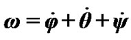
According to the theorem of momentum relative to moving center of mass [14], the rotational motion of a mechanic system is described as the law of angular momentum change:
 (1)
(1)
where  is the angular momentum of a mechanic system relative to the center О in the non-rotating coordinates x1y1z1 (Figure 1), and
  is the moment of the applied force
  relative to this center in the same coordinates.
We provided а number of experiments (Figure 1) to understand better the mechanism of gravitation force action on a rotating body. Let a whirligig (Figure 1(a)) rotates on a table. Having its own axis counterclockwise inclination from a vertical at the angle , it is treated by gravitation force
  creating the moment of force
 , which is counterclockwise also. In case of the suspended wheel (Figure 1(b)) the torque
  will be clockwise. Experiments were executed at different
  angles and angular speeds of these bodies. Direction of precession of the whirligig and a suspended wheel axes were opposite in all experiments.
Now we consider the law of angular momentum (1) on an example of rotational movement of three bodies submitted on Figure 1 in more details. Let a whirligig (Figure 1(a)) be at angle  to the axis z1 and spin about its axis z at the angular velocity
 , and the gravitational force
  be applied to its gravity center. The torque
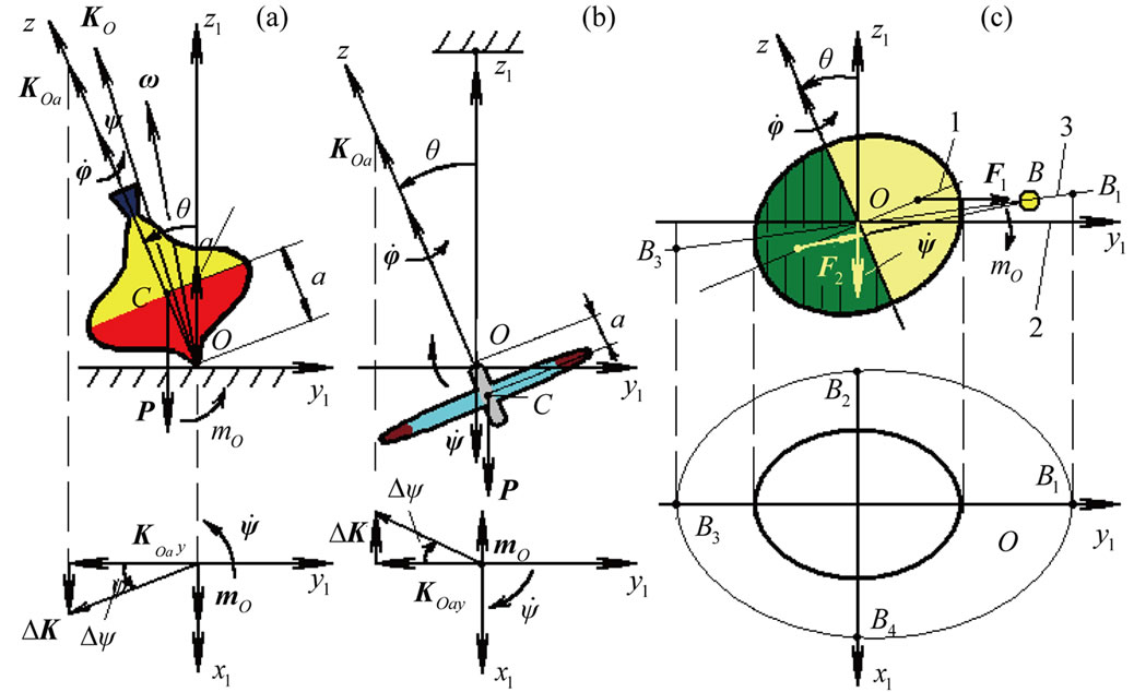
Figure 1. Precession of rotational bodies: (а). Whirligig on bearing surface x1Oy1; (b). Wheel suspended at the point O; (c). Free Earth. 1 and 2—Earth’s equatorial and orbital planes; 3—orbital plane of the body B.
(moment of force)  makes the whirligig axis rotate about the point O at the angular velocities
  and
and . The vector of the whirligig absolute angular velocity is
 (2)
(2)
Let a axisymmetrical whirligig with the moment of inertia Jz relative to z has the velocity  which is much faster than the velocities of its axis
  and
and . If we neglect the deviation of
  from z (Figure 1(a)), the whirligig approximate angular momentum
 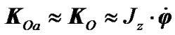 is directed along z, and law (1) becomes written approximately as
 (3)
(3)
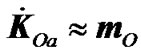
This approach is employed in the elementary gyroscope theory. The torque  being normal to
  (Figure 1(a)), the angular momentum remains invariable in magnitude
 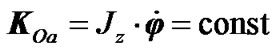 but changes its direction
  in the plane x1Oy1 according to
 . Then, for the time
 , the angular momentum receives the increment
 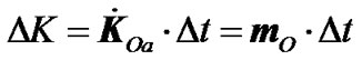 which causes its rotation with the angle
  about z1. If the increment ΔK is expressed via the angle increment
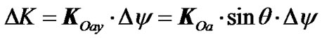 the rotation velocity becomes
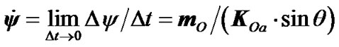 (4)
(4)
Inasmuch as the whirligig spin axis coincides with the angular momentum  in this formulation, it will rotate in the same way as
 , i.e., will precess counterclockwise at the velocity
 . After the moment
  is substituted into (4), the precession velocity becomes
 (5)
(5)
In the applied approximation, the precession velocity does not depend on the tilt of the whirligig spin axis  and moreover, there are no nutation oscillations (changes of angle
 ).
).
In case of a wheel suspended at the point O (Figure 1(b)),  is directed clockwise, and the wheel axis precesses also clockwise at a velocity governed by (5).
Figure 1(c) shows the action of body B on the rotating Earth. If the Earth is centrosymmetrical, the action of B on the Earth’s parts nearest and farthest to B corresponds to the forces  and
and , whose resultant passes through the center O. For an oblate Earth, the purchases of these forces become farther from the center O. Then,
  increases while
  decreases producing the torque
  directed clockwise as in Figure 1(b). Therefore, the Earth’s spin axis will processes clockwise at a velocity given by (4).
Above we considered the rotation at an angular velocity , i.e. counterclockwise. If the rotation changes its direction from counterclockwise to clockwise, the precession changes correspondingly, i.e. the velocity changes sign. It was proved by experiments.
It is possible to establish the precession cycles of the Earth’s spin axis by analyzing the action body B on Earth (Figure 1(c)). The body B produces the maximum torques  of the same direction at points B1 and B3, which are zero when the body is in the Earth’s equatorial plane (B2 and B4), i.e., the torque changes twice from 0 to
  during a single orbiting cycle of B. Therefore, the precession and nutation cycles of the Earth’s spin axis equal the half orbiting periods of the Sun, the Moon, and the planets relative to the moving Earth’s axis Oz, or to the moving equatorial plane.
The Earth and the planets may approach in their orbital motion. If the approachment occurs at the points B1 and B3, the maximum torque increases to . Thus, the Earth’s axis oscillates with periods corresponding to cycles at which the Earth approaches with planets are especially the closest to it at the points B1 and B3. Note, that with the purpose of simplification Figure 1(c) the three planes are shown with intersection at line B1B2: 1 and 2—Earth’s equatorial and orbital planes, 3—orbital plane of the body B. Therefore these oscillation periods are modulated because the orbits of the Earth and the planets do not belong to the same plane and are rather elliptical than circular.
The torque produced by body B, depends also on parameters of its orbit, in particular from a tilt between the equatorial plane 1 (Figure 1(c)) and the orbital plane 3. Therefore the Earth’s spin axis will oscillate with the period of orbit precession of the body B relative to the Earth’s moving equatorial plane. For example, the precession cycle of the Moon’s orbit relative to the Earth’s orbital plane is equal 18.6 yrs. The Earth’s spin axis will oscillate with this cycle at the Moon action. There will not be an essential difference between this cycle and the cycle of the Moon’s precession because the precession cycle of the Earth’s equatorial plane exceeds the last one in more than thousand times, i.e. during the cycle of the Moon’s orbital precession the Earth’s equatorial plane is practically motionless.
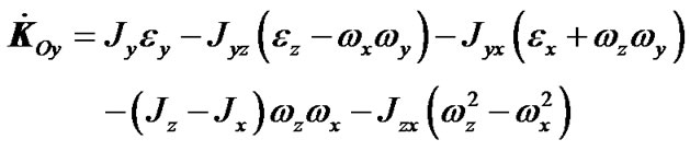
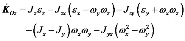
3. Differential Equations of Rotational Motion
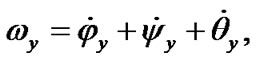
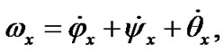
3.1. Earth’s Angular Momentum
There arises a problem in the derivation of the rotation equations: as the body rotates the moment of inertia or the angular velocity components are changed depending on the coordinate system. Therefore, we first use the coordinates in which the moments of inertia remain invariable and then we proceed to the coordinates where the angular velocities are independent of the body rotation.
Motion of the Solar system bodies is considered in non-rotating barycentric ecliptic coordinates x10y10z10 (Figure 2) connected to the Earth’s orbital plane fixed at T0 epoch. Axis x10 is pointed toward the vernal equinox. Let the non-rotating system of geocentric ecliptic coordinates x1y1z1 with the center of mass at O moves translationally relative to the system x10y10z10. Axis z of the rotating geocentric ecliptic coordinates xyz is directed along the Earth’s own angular velocity  and axis x at the initial moment t = 0 lies in the Greenwich Meridian plane. The Earth’s absolute angular velocity
  in system x1y1z1 with the projections ωx, ωy, ωz to rotating axes of system xyz will be
 .
.
In the law (1), angular momentum  is produced by all the masses of rotating Earth in system x1y1z1, and
  is moment of forces produced by all the Solar system bodies. First define derivation of the angular moment and then the sum of torques.
As in system x1y1z1 the Earth rotates with angular velocity , thus any of its element dM with a radius vector
  (Figure 2) moves with velocity
  and has angular momentum
 relative to the center O.
After integration taking into account the entire Earth’s mass M,  is
is
 (6)
(6)
Having differentiated  on time and then having substituted vectors
 ,
,  and
and , after transformation we obtain derivatives of the projections of the angular momentum to axes of rotating system xyz
 (7)
(7)
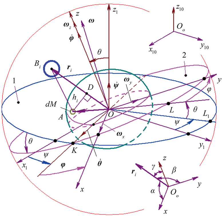
Figure 2. Coordinate systems and action of the body B on the Earth’s element dM: x10y10z10—fixed barycentric ecliptic system; x1y1z1—non-rotating geocentric ecliptic system; xyz —rotating with Earth geocentric equatorial system. ,
,  and
and  are Euler angles of position of system xyz relative to system x1y1z1. 1—fixed ecliptic plane; 2—Earth’s moving equatorial plane;
 —radius vector of mass element dM relative to center O.
 (8)
(8)
 (9)
(9)
where εx, εy, εz are projections of the Earth angular acceleration in system x1y1z1 to axes of rotating system xyz;
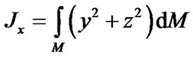 ,
, 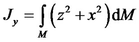 ,
,  —the Earth’s axial moments of inertia, and
 —its centrifugal moments of inertia.
As the system xyz is connected with the rotating Earth, the moments of inertia do not depend on the Earth’s rotation and remain constants. Today’s knowledge of the Earth’s density distribution is insufficient for definition of the moments of inertia. As it will be shown below, it is possible to define only the relation between two moments of inertia Jz and Jx, from observable angular velocity  (precession), but not their absolute values. Last years the three-axial model of Earth is described where the third moment of inertia is estimated by potential of the gravitational distribution on Earth’s surface. However, this method can not give precise estimation of the moments of inertia. Note, that in case of three-axial Earth it is required to add terms with centrifugal moments of inertia because of nonsymmetrical distribution of potential as shown from (7)-(9). Traditionally, terms with these moments are unaccounted and terms containing third moment Jy are in equations though in last forms Jy is equal Jx. Nevertheless, avoiding of complications with unaccounted terms it is considered axisymmetrical Earth Jy = Jx, and Jxy = Jxz = Jyz = 0. Then derivatives of the angular momentum (7)-(9) are:
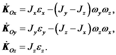 (10)
(10)
For axes with zero centrifugal moments of inertia the moments Jx, Jy, Jz are named principal moments of inertia.
3.2. The Law of Angular Momentum in Euler Angles
Position of rotating system xyz (Figure 2) relative to non-rotating system x1y1z1 is determined by Euler angles: ,
,  ,
,  , here precession angle
  defines position of nodes line OK, where moving equatorial plane intersects fixed orbital plane (ecliptic), nutation angle
  defines a tilt between equatorial plane and ecliptic and
  is angle of the Earth’s own rotation around axis z. Figure 2 shows directions of this angles accepted in theoretical mechanics. In astronomy angles, which are directed according to observably movements, are accepted:
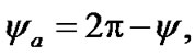 and
and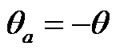 . Directions of angular velocities

 are shown on Figure 2, i.e. turn of angles
 ,
,  and
and  is visible counterclockwise from the side of these vectors. It is seen from Figure 2 that Euler’s velocities stay constant at the Earth’s turn. Therefore let all the variables and equations will be expressed in Euler variables.
As it is possible to present the vector of absolute angular velocity as (2), thus in projections to axes x, y, z it is
(11)
where 

 etc. —projections of the Euler angular velocities to axes xyz. Having calculated expressions (11) with the help of Figure 2 it is received Euler well-known equations:
 (12)
(12)
After differentiation (12) the angular accelerations in Euler variables become:
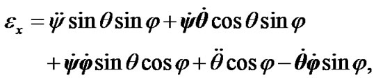 (13)
(13)
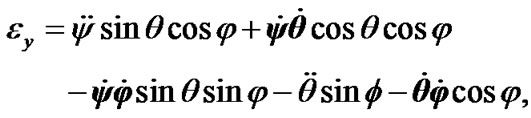 (14)
(14)
 (15)
(15)
Having substituted angular velocities (12) and angular accelerations (13)-(15) in (10), the projections of derivatives of the angular momentum depending on Euler angles are:
 (16)
(16)
 (17)
(17)
 (18)
(18)
Let us transform the law of the angular moments (1) to Euler angles. The moments of forces can be defined directly through forces for the actions of each body on an Earth mass element (see Figure 2). However, hereinafter at their series representation they are reduced to other terms. Here we define the moments through the force function U by a traditional method to safe continuity with previous works. As it is known from the theorem of theoretical mechanics, the moments of forces in a direction of axes are equal derivatives of force function on an angle of turn relatively to this axis. Therefore in system OKz1z with the axes located on vectors of angular velocities 
 and
and , the moments of forces are (Figure 2):
 . Taking into account these moments we project the right and left part of (1) on the axes of system OKz1z:
 ,
, 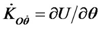 ,
,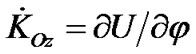 (19)
(19)
Let us express derivatives of the angular momentum in Equation (19) through derivatives ,
,  and
and  in Cartesian coordinates Oxyz, and draw axis OL perpendicularly to axis OK (Figure 2).
Then, projections of the derivatives ,
,  and
and  (on Figure 2 are not seen but identical to projecttions
 ,
,  и
и ) on axes of system OLKz1 are
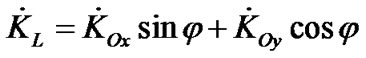
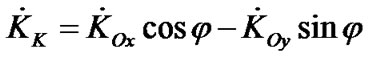
and then:
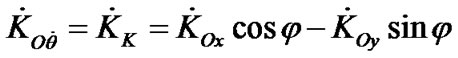 (20)
(20)
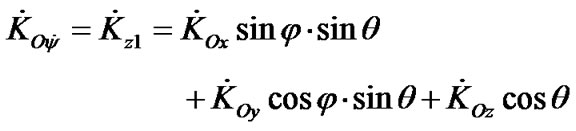 (21)
(21)
Further the Cartesian projections (16)-(18) are substituted in Equations (20) and (21), and the last ones are substituted in (19) in system OKz1z. Then, having expressed the second derivatives it is received two differential equations of the Earth’s spin in Euler’s variables:
(22)

(23)
where the derivative of the angular momentum  is defined by the third formula in the Equation (19) for the law of angular momentum.
3.3. The Force Function in Cartesian Coordinates
Now we define force function for the action of body Bi with mass Mi (Figure 2) on the Earth by the traditional way presented, for example, in [15]. Its coordinates in rotating system xyz are xi, yi, zi. The force function of the action of this body on the Earth’s element of mass dM with coordinates x, y, z is  where G is the gravitation constant,
 is the distance between the element of mass dM and the body Bi. Having summarized on all Earth’s mass M and on all bodies n the force function is:
 (24)
(24)
where 
 is the Earth’s density.
It is obviously impossible to integrate Equation (24) because today’s distribution of the Earth’s density is studied only qualitatively. Therefore direct definition of the force function for the action of external bodies on the Earth as mechanical system is impossible. All further solutions are in simplification of Equation (24) and in derivation of the force function depending on the Earth’s moments of inertia Jx, Jy, Jz. Correlation between them are defined on observable rate of the Earth’s precession.
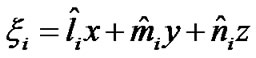
Taking into account that the distance ri between the Earth and the body Мi is considerably exceeds distance r to the element dM the Equation (24) is simplified. Let the line segments OD = ξi and AD = hi. Having applied the theorem of Pythagoras to cathetus hi of both rectangular triangles ΔODA and ΔADBi, we obtain:
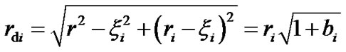 (25)
(25)
where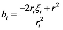 .
.
As  then subintegral function
  in (24) is represented as Taylor series at b powers. Taking into account terms that are no more the fourth order in relation to
 , the force function is in form
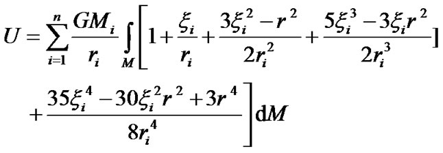 (26)
(26)
Line segment  (Figure 2) is expressed through coordinates x, y, z of the element dM by means of direction cosines

 :
:
 (27)
(27)
where
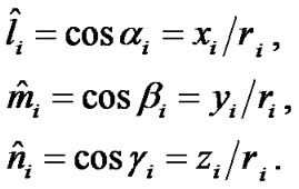 (28)
(28)
By definition, the axes of a body, which are on intersection of planes of symmetry, are the principal axes of inertia. Axes of rotating system Oxyz are directed along the Earth’s principal axes of inertia. Therefore integrals of type 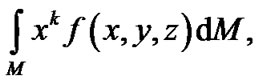 where k—an odd integerand
 —even function of coordinates, will consist of two equal on size and opposite on a sign parts at the intervals
  and
and , i.e. these integrals are equal zero in the sum. Because, according to (27), variable
  is proportional to coordinates x, y, z, the integrals in (26), depending on
  and
and , are equal zero. Note, that these integrals are necessary to consider in case of the non-symmetrical Earth and absence of symmetry on one of the planes zOx or zOy, i.e. the force function as well as the derivatives of angular momentum (7)-(9) will include centrifugal moments of inertia.
Integral of the first term in (26) is the Earth’s mass. Numerator of the third term with the account (27) is
(29)
As  thus in (29) it is taken into, that
 . The terms integration having coordinates in the second power gives the moments of inertia and the last ones gives centrifugal moments as
 which are zero for the Earth with princepal axes along x, y, z.
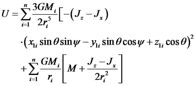
After substitution (29) in (26) and integration we obtain the force function without the last fifth term
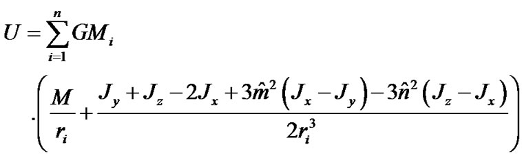
(30)
In this case the action on the Earth’s rotational motion is defined by the third and the fifth terms in (26) as they depend on Euler angles. Having divided the fifth term on the third, we find that the order of their relation is equal  where RE—radius of the Earth. This ratio has the greatest value for the Moon, and is equal 3×10⁻⁴. Further the bodies’ action on the Earth’s spin is considered with such relative error. Therefore additional effects should be considered, if the relative value of their action has the order 3×10⁻⁴ and more.
After the direction cosines  and
and  are substituted according to (28), force function (30) becomes
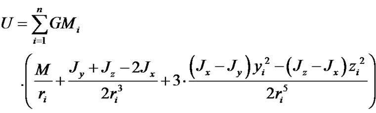
(31)
where yi and zi—coordinates of the body Mi in rotating system xyz.
3.4. The Moments of Forces in Euler Angles
We express yi and zi through coordinates x1iy1iz1i of system x1y1z1 (Figure 2). Let us draw the line OL1 perpendicularly to OK in the plane x1Oy1. Coordinates of the body Bi will give projection 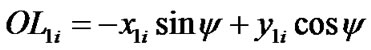 on this line and then coordinate z of the body Bi is
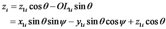 (32)
(32)
Having defining projections of the coordinates x1i and y1i to the axes OK and OL analogously, coordinate yi is
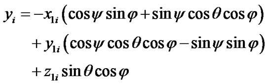 (33)
(33)
Earlier we neglected the centrifugal moments of inertia. It is admissible, if the Earth is axisymmetrical, or axes x and y lie in symmetry planes. As there is no evidence on presence of such planes we should consider the axisymmetrical Earth with the equal moments of inertia relative to axes x and y, i.e. Jy = Jx. Therefore we do not present bulky expressions for the non-axisymmetrical Earth. If necessary they may be received on below-mentioned sequence with use of expression (33). For the axisymmetrical Earth, after substitution (32) in (31), taking into account Jy = Jx, force function becomes:
 (34)
(34)
After differentiation (34) on Euler angles φ, ψ, θ and reductions we obtain the moments of forces
 (35)
(35)
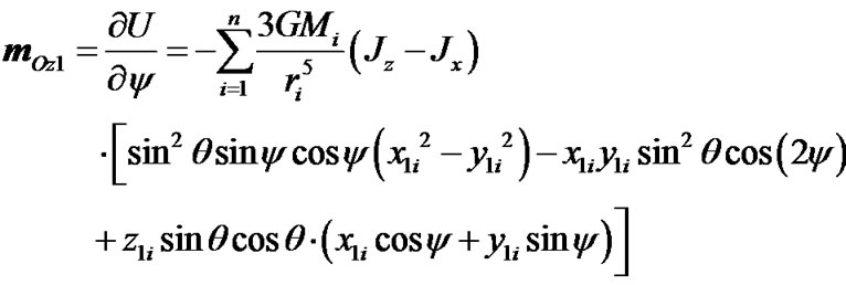
(36)
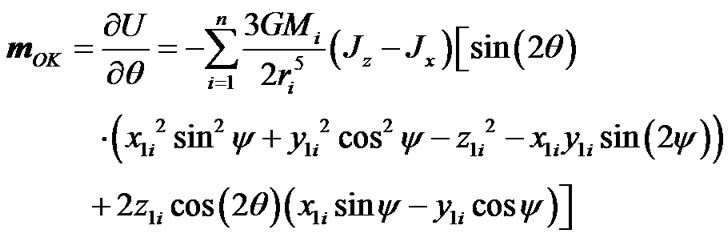
(37)
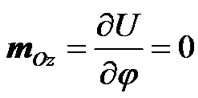
3.5. Differential Equations
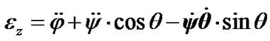
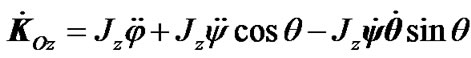
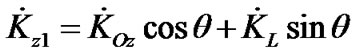
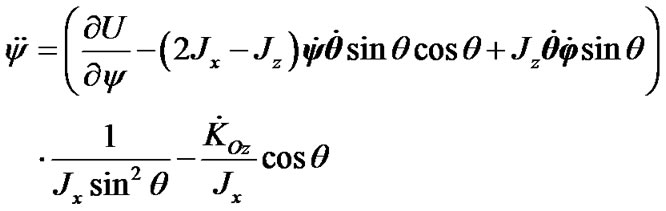
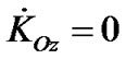
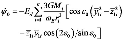
The law (1) in projection to the axis z of rotating system xyz, according to (19), has a form . We consider the rigid Earth during derivation of the equations: Jz = const. The moment of inertia of the axisymmetrical Earth JOz may be changed for the action of redistribution of a water cover, thawing of glaciers, moving of continents, etc. In order to estimate the influence of these factors, it is entered Jz ≠ const. Therefore, according to (35)
 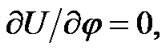 then
then  and taking into account (10) at Jz = Jz0 it becomes
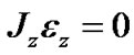 . After integration it is
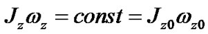 , that may be written in form
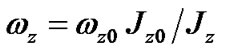 (38)
(38)
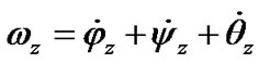
where Jz0 and ωz0 are the Earth moment of inertia and its projection of angular velocity in an initial epoch. Because 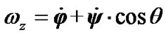 (according to Equation (12)), thus, taking into account (38), we obtain angular velocity of the Earth’s own spin
 (39)
(39)
From expression (39) follows that angular velocity of the Earth’s own spin , which is not connected with motion of vector of angular speed
 , may be changed via redistribution of the Earth’s moment of inertia and alteration of precession rate. Expression (39) for angular velocity of the Earth’s own spin may be used for an estimation of the Earth’s parts motion influence on its angular speed.
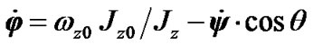
Having designated a projection of the Earth’s angular velocity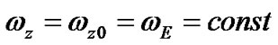 , expression (39) for the rigid Earth
 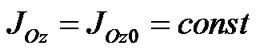 we rewrite in a kind
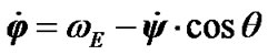 (40)
(40)
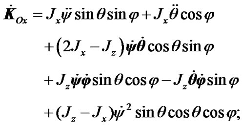
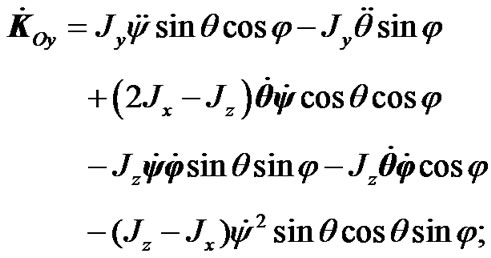
After substitution of ,
,  and the derivatives of the force function (36) and (37) in Equations (22) and (23), differential equations of the Earth’s rotational movement are
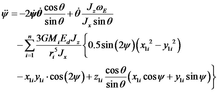
(41)
 (42)
(42)
where 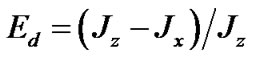 is the Earth’s dynamical ellipticity;
  projection of the Earth’s absolute angular velocity to its axis z, and ratio of moments is
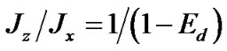 .
.
As  = const and
  changes according to (40), thus value
  may be obtained as a result of averaging of the measured values
  и
и on time, i.e.
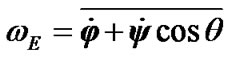 .
.
4. Initial Conditions and the Earth’s Dynamical Ellipticity
We study the action of separate bodies on the Earth, therefore at integration Equations (41) and (42) it is necessary to set initial values for alteration of rates  and
and , which are determined by influence of each body. At any set of initial values
  and
and  there begins a transient response, which may become whether a steadystate regime in a long time or not to be steady state at all. We are interested in the Earth’s behavior at steady-state regime. Let the second derivatives
  and
and  in Equations (41) and (42) are small in relation to the other terms at steady-state regime, i.e.
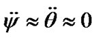 . As
. As  exceeds the derivatives
  and
and  on 6 orders therefore at neglecting terms with
  and
and  in Equations (41) and (42) they become
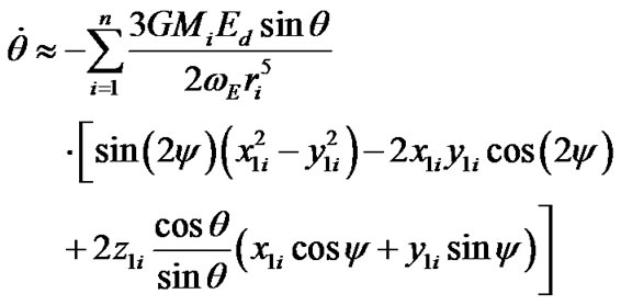 (43)
(43)
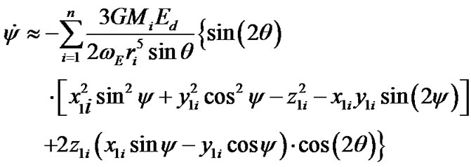 (44)
(44)
Equations (43) and (44) are identical to the Poisson equations; their approximate solutions are applied in astronomical theories of climate change. We will define initial values of derivatives from these equations, setting coordinates x1i, y1i and z1i of bodies acting on the Earth during an initial epoch t = 0. Initial values of the angles are:  and
and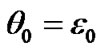 , where
  = 0.4093197563 is the inclination due to an initial epoch, for example 30.12.1949.
There is the unknown parameter , which defines relation between the Earth’s moments of inertia. Today’s knowledge of the Earth’s density distribution is insufficient for definition of the moments Jz and Jx with a demanded accuracy. Therefore the Earth’s dynamical ellipticity Ed is defined by comparison of the calculated precession rate with the observations. According to [16,17] the Earth’s precession has clockwise direction relative to the fixed ecliptic and during a tropical year is
 (45)
(45)
where T is counted in tropical centuries from a fundamental epoch 1900.0 with JD = 2415020.3134. In an initial epoch it is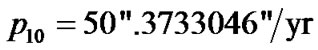 . Observable average precession rate is described by Equation (45). Now we define its calculated value according to (44). If an initial epoch coincides with an epoch of reference frame, then
  and
and . Then Equation (44) is written
 (46)
(46)
where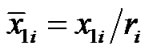 ,
,  ,
, —dimensionless coordinates of acting bodies.
If a reference epoch does not coincide with an epoch of reference frame,  , and
, and .
.
In the course of cyclic relative movement of bodies round the Earth all coordinates change similarly, for example . Hereat
 , and
, and , where ii—the tilt between the body’s orbital plane and equatorial plane. Since Pluto has the most value of the tilt ii = 0.7 [6], for all planets
 . The second term in a square bracket (46) will change in limits
  and averaging on time will make it zero. The maximum value of the factor of the first term
  is 1, and minimum is zero, therefore and averaging on time will give 0.5. Then all the part in square brackets at averaging is
 .
.
Value of geocentric distances to the planets changes in limits , where
 ,
,  and
and ,
, —perihelions and afelions of the planets and the Earth, accordingly. Then average geocentric distance to the planets is
 (47)
(47)
which is  for internal planets, and
  for external, where ai, aE and ei, eE—semimajor axes of heliocentric orbits and orbits eccentricity of the planets and the Earth accordingly. Accordingly, for the Sun and the Moon average geocentric distances are
 ,
, (48)
(48)
where aM—average semiaxis of the Moon’s orbit. Then average value of speed of precession, according to (46), one gets
 (49)
(49)
The negative sign testifies clockwise direction of precession. Due to equality condition between calculated average precession rate and observed one , where
 —duration of a sidereal year in sec, and
  we find the dynamical ellipticity
 (50)
(50)
where index a and Eda denote approximate method of calculation of this value.
Having derivated Equations (49) and (50) we averaged enough approximately expression (46) on time, for example, the average values  and ri can essentially differ. If laws of planets motion x1i(t), y1i(t), z1i(t) could be found, there were known average value
  on time span T by integrating expression (46) on time at interval from 0 to T. However, expression (46) is approximate since it is obtained from the equations of motion at neglecting
  and
and . Therefore Equation (50) represents the Earth’s dynamical ellipticity approximately. Its more exact value will be obtained after numerical solution of the Earth’s rotational movement Equations (41) and (42) and comparisons of averaged from short-period oscillations of dynamics
  during known observation with observable dynamics of average precession for this period.
The value of dynamical calculated according to (50) under the data used by us, is Ed0 = 3.324257·10–3. Traditionally dynamical ellipticity is calculated with the account only the Moon and the Sun. In this case, under our data EdSM1 = 3.324268·10–3 i.e. differs at unit of the sixth positional notation. As it is seen from (50), the dynamical ellipticity depends on averaged distance , thus the small changes of its value sufficiently change Eda.
For instance value of this distance for the Moon , which we obtained at reference conditions at epoch 30.12.49 from ephemerides DE406, gives dynamical ellipticity EdSM2 = 3.324770·10–3. To comparison here are ellipticities used by various authors: Bretagnon and Simon [11] EdB = 3.2737671·10–3; F. Roosbeek and V. Dehant [18] Ed = 3.273767·10–3; Laskar et al. [5] Ed = 3.28005·10–3 with using aM = 384747980 м and p10 = 50.290966''/yr.
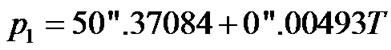
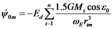
As we see, values Ed in expression (50) change depending on the accepted data in the second significant figure. The value dynamical ellipticity, taking into account the data accepted by us, is designated as Ed0, and according to Simon et al. [19] as EdS. Table 1 gives Earth’s axis mean precession rates for the action of the Sun, the Moon and the planets calculated according to (49) and Ed = EdS. The most value of speed of precession is caused by the Moon, the action of the Sun is twice less, and Venus and Jupiter cause the greatest action from the planets. As it is seen from Table 1, difference between speed of precession  for the action of all the bodies and observable value p10 is 3.14·10–3%.
Due to accepted dynamical ellipticity EdS and ,
,  , initial values
  and
and  are calculated according to (43) and (44) for the action of the separate bodies and all together, see Table 1. Note, that expressions (43) and (44) represent values of derivatives
  and
and  approximately. Their exact value is given by observation. There are no these values for the action of separate bodies but there are observation data for the simultaneous action of all the bodies on the Earth. However, as Equations (43) and (44) are approximate, total values
  и
и (taking into account all the bodies) will differ from the observation data.
5. Solution Algorithm
The coordinates x1i, y1i, z1i of the bodies Mi, acting the Earth in Equations (41) and (42) are referred to the fixed geocentric ecliptic coordinates (Figure 2). Numerical solution of the orbital problem gives the change of their orbit parameters i, φΩ, φp, Rp, e over a time span 100 Myr [6]. Due to this solution there are the bodies’ positions saved with 10 kyr interval. To integrate equations of rotational motion one needs the bodies’ positions during any moment of time.
The bodies’ positions are usually set on the base of the theory of secular perturbations during solving rotational motion equations. Bretagnon et al. [11] used ephemerides DE403 for numerical integration of these equations for 1968-2023 yr interval. These methods are not suitable
Table 1. The mean precession rate  of the Earth’s axis and the initial rates
  and
and  for the separate action of the bodies by results of computations according to (49) and (43)-(44), accordingly. Computations executed at EdS = 3.2737752·10–3; p10 = 2.4422·10–2 rad/cyr;
 ;
; ; rad in radians and cyr in centuries years.
for long-time integration. Therefore we developed the follow algorithm to compute the motion laws of the bodies x1i(t), y1i(t), z1i(t). Their coordinates are defined on the base of our solutions about motion of the Solar system bodies in fixed barycentric equatorial coordinates. Using orbital parameters i, φΩ, φp, Rp, e Cartesian coordinates are recalculated in polar ri and φi in orbital plane. To estimate the body position during new moment of time t1 = t+Δt one may use expressions for elliptical motion given in [12,13,20,21]: t = t(r)—motion law in implicit form and r(φ) – trajectory equation. Polar radius of the body r1 during new moment of time t1 is predicted under Taylor’s formula of the second order, checked on dependence t1(r1) and then discrepancy for some iterations comes almost to zero. After that from the trajectory equation there obtained polar angle φ1(r1) in a return form. At small ellipticities e - 0 during new moment of time t1 under Taylor’s formula the angle φ1 is predicted, checked under the movement law t1(r(φ1)), then the discrepancy for some iterations also practically comes to zero.
This algorithm differs from the traditional. The intermediate parameters: mean anomaly M and eccentric anomaly E, which feature in traditional description of body motion on an elliptic orbit, are not used here.
The bodies polar coordinates r1, φ1 during any moment of time are recalculated in coordinates of translationally moving geocentric system x1y1z1 via orbital parameters i, φΩ, φp, Rp,. Since the orbital parameters change from one epoch to another, they are interpolated on a parabola on each step. Thus, the algorithm, which allows defining the bodies coordinates xi, yi, zi acting the Earth at any moment from the considered interval of time, is developed. Note, that the Moon’s orbit has more short oscillation periods comparably with the other orbits of planets. Therefore the algorithm for the Moon was modified upon with their account.
We applied the Runge-Kutta integration of Equations (41) and (42). These algorithms of calculation of coordinates and numerical integration are programmed on the FORTRAN. The computation was run on personal computers and supercomputers MVS-1000 at Keldysh Institute of Applied Mathematics of the Russian Academy of Sciences (Moscow) and NKS-30T at Siberian Branch of the RAS Computing Center (Novosibirsk). As a result of numerical experiments we accepted the initial integration step  = 1×10⁻⁴ yr.
6. Numerical Integration Results
6.1. The Sun’s Action
Figure 3, a gives results of integration Equations (41) and (42) over 0.1 yr for the action of the Sun on the Earth’s rotational motion. The precession angle  decreases since zero value making fluctuations with the amplitude
  = 6.53·10–8 rad = 13.47 mas and the period T1 = 0.99348 d, where: mas is 10–3 angular seconds, d is duration of a day in sec. The nutation angle is presented as difference
 , where θ0 = 0.4931976 rad. As it is seen from the graph
  value of the tilt between moving equatorial plane and fixed ecliptic increases, making fluctuations with amplitude
  = 2.60·10–8 rad = 5.27 mas and same period T1. Rate of precession
  oscillates round some mean value with period T1 and amplitude
  = 1.57·10–2 rad/cyr. Rate of nutation oscillates with the same period T1 and amplitude
  = 6.17·10–3 rad/cyr round almost zero value.
As it is seen from Figure 3, a initial values of the rates  and
and  do not exceed their extreme values. Therefore an error in definition
  and
and  causes only change of an initial phase of fluctuations. Hence, in this case dynamics of the rates
  and
and  is not changed at an error of initial conditions described in p. 4. There are similar properties of solutions for the action of other bodies, thus this property will be kept for the action of all bodies. Consequently, the initial conditions in this case calculated according to (43), (44), may be specified on a phase of observed daily oscillations
  and
and .
.
As the accepted initial conditions, according to (43), (44), are artificial, there arises the question. Which values of derivatives  and
and  might be, if a long-time action of a single body on the Earth preceded the begin- -ning of calculation? Apparently, there would be an occurrence of equilibrium and derivatives would come nearer to the mean values. With this purpose there were defined mean values
  = 1.61891·10–2 and
  = –1.32398·10–3 according to the first daily oscillations (see Figure 3(a)). Integrating Equations (41)-(42) with initial values
  and
and  has resulted in reduction of daily oscillations in 20 times (see Table 2). Hereat character of solutions behavior for the long-time actions has not changed.
At averaging derivatives in new solutions there obtained mean values  = 1.59342·10–2 and
  = –1.08328·10–3, submitted in Table 2. Repeated calculation with these initial values has resulted in diminution of amplitudes of oscillations in several times. Thus, there were executed 4 calculations with specification of the mean values of initial rates. Consequently, amplitudes of daily oscillations have decreased in several hundred times, according to Table 2.
It is possible to account the final values of derivatives  and
and  as steady-state for long-time action of a single body on the Earth. For the action on the Earth
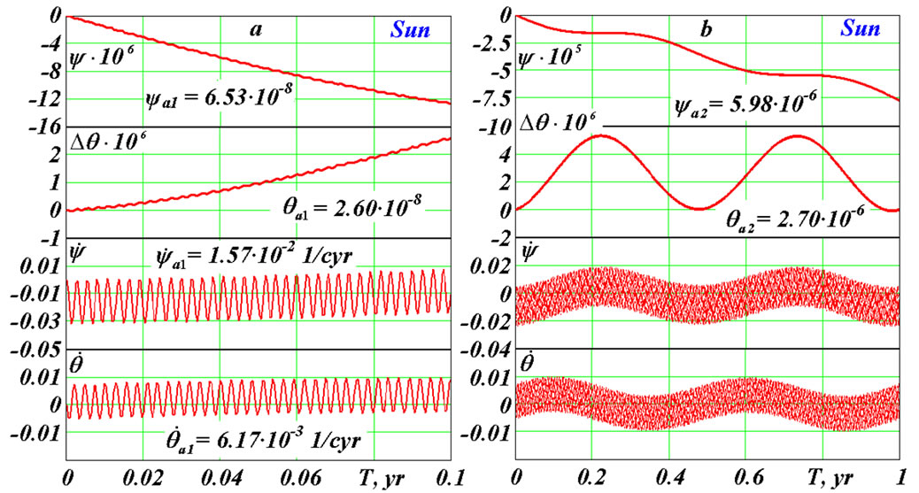
Figure 3. Action of the Sun on the Earth’s rotation: a – during 0.1 yr; b – during 1 yr. Precession angle  and nutation angles difference
  are in radians and rates
  and
and  are in radians per century; T—begins with initial epoch 30.12.1949.
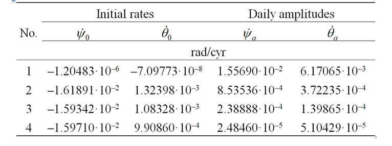
Table 2. Amplitudes of daily oscillations for the action of the Sun at specification of the steady-state initial rates.
several bodies there, apparently, will not be such steadystate condition for each body. Therefore further we consider the action of single bodies at initial conditions, according to (43), (44).
Figure 3(b) shows the Earth’s axis dynamics for 1 yr. The precession angle increases clockwise making oscillations with period T2 = 0.5 yr and amplitude  = 5.98·10–6 рад = 1232 mas. The nutation angle oscillates with the same period T2 and amplitude
  = 2.70·10–6 рад = 556.9 mas around mean value. A minimum of the Earth’s inclination is in the reference epoch (30.12.1949). It is explained by the most deviation of the Sun from the equatorial plane, which makes the most moment of force giving
 .
.
Figure 4(a) presents axis dynamics for 10 yr. The precession angle  changes practically linearly with semi-annual oscillations marked earlier, and the nutation angle with the period T2 oscillates about mean value. The rates
  and
and  with the periods T1 и T2 change in the same bounds, as on Figure 3(b). The Earth’s axis dynamics over 100 yr is shown on Figure 4(b). The precession angle
  changes linearly with mean rate
  = 7.74·10–3 rad/cyr during 1000 yr. The nutation angle in the form of
  changes with daily and semiannual periods in invariable limits. The rates
  and
and  oscillates also in invariable bounds:
  around the mean value
 , and
, and  around almost zero value. The parameters behavior over 1000 yr is the same, therefore these results are not submitted here.
Obtained as a result of integration (41), (42) the mean value of precession rate coincides with the mean value  = 7.73·10–3 rad/cyr calculated on the approximate dependence (49), (Table 1). It is necessary to notice that the instant precession rate (Figure 3(b)) changes in bounds
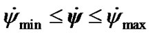 , where
  = 0.016 rad/cyr, and
  = –0.032 rad/cyr, i.e.
  changes more than in 20 times relative to an average. The rate
  changes in more relative bounds in relation to its mean value
 . However, at such considerable changes of the instant rates
  и
и the mean values remain constants during all integration interval. It testifies stability of the integration method. And as mean values
  correspond with observations, it testifies reliability of the solution of the entire problem.
Note, that under consideration of the action of the body B on the Earth (Figure 1) there was shown that the torque m0 < 0 and the precession rate  < 0. As a result of integration (41), (42) we have received that precession rate takes positive values also (Figure 3(b)). This result is caused by dynamics: under the action of torque the Earth’s axis speeds up, according to (4), and its motion proceeds even in absence m0 due to inertia. Therefore
  is more than the value given by (4), and
  > 0.
> 0.
Here we do not submit graphs of the Earth’s angular velocity dynamics , since, according to (40), the hanges of
  have contrary sign to the changes of the precession rate
 . This conclusion is proved by results of other authors, for example, [9].
6.2. The Moon’s Action
The moon has the strongest action on the Earth’s axis dynamics. Figure 5(a) gives the daily oscillations of the parameters with the period T1 = 0.99348 d and amplitudes  = 7.29·10–8 rad = 15.04 mas,
  = 2.83·10–8 rad = 5.83 mas,
  = 1.66·10–2 rad /cyr and
  = 6.63·10–3 rad/cyr. Against daily oscillations there appear half-monthly oscillations with period T2 = 13.5143 d, which are well visible on 1 yr interval (see Figure 5(b)). The precession angle has a linear trend and also oscillates with the half-monthly period and amplitude
  = 1.16·10–6 рад = 240.10 mas. For 10 yr interval the parameters behave analogically, therefore these results are not submitted here.
The further changes of parameters we will consider for 100 yr interval (Figure 5(c)). Here there are new oscillations with period T3 = 18.6 yr. Along with linear the change of precession angle it has oscillations with the period T3 and the amplitude  = 0.98·10–4 рад = 20286.33 mas. The nutation angle oscillates with this period at amplitude of fluctuations
  = 5.23·10–5 рад = 10797.80 mas.
As it was told in p. 2, due to the analysis of the theorem of momentum the presence of the oscillations caused by orbital precession of the acting body B (Figure 1(c)) has been established. At integration (41), (42) with the Moon action to the Earth, we have obtained oscillations with period T3 = 18.6 yr, which are caused by precession of the Moon orbital axis.
For 1000 yr interval the behavior of the precession  and the nutation
  angles are similar to Figure 5(c). Except oscillations with the period T3 = 18.6 yr others are not present. The mean precession rate is
  = 1.70·10–2 rad/cyr. Oscillations with the period T3 = 18.6 yr also proceed on 10 kyr interval. The trend of change of the nutation angle
  under the cosine law is tracked.
Figure 4. Action of the Sun on the Earth’s rotation: a—during 10 yr; b—during 100 yr. See captions on Figure 3.
Figure 5. Action of the Moon on the Earth’s rotation: a—during 0.1 yr; b—during 1 yr; c—during 100 yr. See captions on Figure 3.
6.3. Action of Venus and Other Planets
Equations (41) and (42) were integrated separately for the action of all the planets. The Venus makes the most influence on the Earth’s axis. Figure 6(a) shows the Earth’s axis dynamics under the action of the Venus on 0.1 yr interval. The precession and the nutation angles oscillates with daily periods and amplitudes  = 2.15·10–12 рад = 0.443·10–3 mas;
  = 0.855·10–12 рад = 0.176·10–3 mas. As we see, the daily amplitudes for the Venus action are in 4 orders less than for the Sun action.
The rates  and
and  also oscillate with daily period T1 = 0.99348 d and the amplitudes considerably exceeding a mean values. As amplitudes of daily oscillations shade oscillations with bigger periods, we do not submit
  and
and  diagrams on the subsequent intervals.
Figure 6(b) represents 10 yr dynamics of the precession and nutation.  change shows that the second period of oscillations with duration about 1.6 yr is tracked. These oscillations are expressed by horizontal lines of the change
 . Their period Т2 = 1.6 yr is caused by periodicity of approach of Venus with the Earth due to their relative motion. Period of these approaches is
 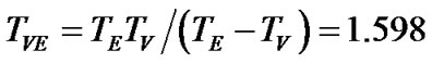 yr, whereе TE и TV are sidereal periods of the Earth and Venus. The graph
  on Figure 7(a) shows 1 cyr interval where oscillations with the period T2 = TVE are made against oscillations with the bigger period Т3 = 8.12 yr and the amplitudes
  = 1.65·10–9 rad = 0.341 mas and
  = 6.16·10–10 rad = 0.127 mas. These oscillations with the period Т3 are caused by periodicity of approach of Venus with the Earth at the longest distance from the equatorial plane (B1 and B3 on Figure 1(c)). Really, after the first approach, for example in the point B1, following approach will be in Т2 = 1.6 yr, i.e. will be aside of the point B2 for 0.1 yr. Therefore 0.5 yr/0.1 yr = 5 approaches, i.e. Т3 = 5·Т2 » 8.1 yr so that the last approach will occur again in the point B1 or B2 is required.
Periodicity of approach in points В1 and В2 can be given by expression
where TBE is the period of approach of the body B with the Earth, and function Int defines an integer part of a number.
Figure 7(b) shows 10 kyr  and
and  dynamics. The angles change linearly with the mean (for 10 kyr) rates
  = –9.53·10–8 rad/cyr and
  = 8.05·10–9 rad/cyr, and the nutation rate is in 12 times less than the precession rate. Difference of the mean nutation rate from zero on 10 kyr interval is caused by the influence of precession of Venus orbital plane relative to the Earth’s equatorial plane during this time. Apparently, further it will
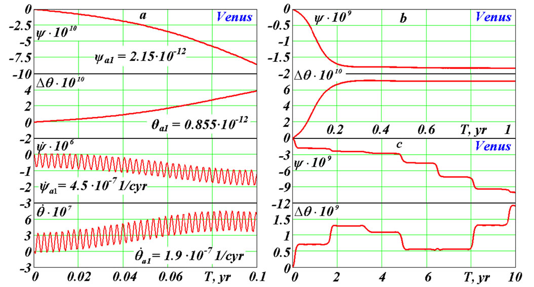
Figure 6. Action of Venus on the Earth’s rotation: a—during 0.1 yr; b—during 1 yr; c—during 10 yr. See captions on Figure 3.
Figure 7. The Earth’s axis dynamics under the action of Venus: a—during 1 cyr; b—during 10 kyr. See captions on Figure 3.
lead to oscillations with a new period.
Graphs of the other planets action on the Earth’s rotational motion look similarly to graphs for the Sun, the Moon and Venus. The most difference proves for the nutation angle. Figure 8 represents the comparison of influence of the Sun and the planets on the nutation angle. Under the action of the Sun, Mercury (Figure 8) and Venus (Figure 7) the nutation angle increases. The action of the other planets leads to its reduction. These changes of the angle  occur, most likely, via the orbital precession of the acting bodies. In the beginning they change linearly for all the bodies (under the sine law), except for the Sun and the Moon. The semi-annual nutation oscillations for the action of the Sun (Figure 4) are big enough and shade the trend
 . Therefore, Figure 8 presents the change of sliding average
  on 100 next points. From the diagram follows that
  changes, apparently, under the cosine law with average rate for 1000 yr
  = 3.3·10–8 rad/cyr.
There are traced different kinds of the nutation oscillations. All the bodies have the daily oscillations with the period Т1. Oscillations with the semi-orbital period Т2 are brightly expressed for the Sun and external planets, except for Pluto, which has the oscillations  with the period 2Т2. For near planets from Mercury to Mars there are oscillations having horizontal maxima with orbital periods ТBЕ of the bodies (B) relative to the Earth (E), for example, 1.6 yr for Venus and 2.14 yr for Mars. Horizontal parts of graphs of the angle
  are caused by long contact of the planet and the Earth during approach. There are brightly expressed oscillations with the period Т3 = ТВС = 8.1 yr for Venus, which are caused by approach with the Earth in the points В1 and В2. For Mars the doubled periods with Т3 = 2ТВС. = 2·7.9 = 1.58 yr are received. The cause of the periods doubling is the result of that the action of the bodies in diametric opposition points relative to the Earth differs due to eccentricity of the orbits and their inclination to the equatorial plane. Therefore the action in one of the points becomes prevailing, thereby the period of oscillations is fixed on it.
The periods and the amplitudes of the Earth’s axis oscillations and the rates of precession  caused by the action of the Sun, the Moon and the planets are given in Table 3. The Moon acts mostly on the amplitudes and the precession rate. Venus renders the most action among the planets.
Having comparing precession rate  with the mean value
  calculated under the Equation (49), it is visible (Table 1) that they are close for the Sun, the Moon and the far planets from Jupiter to Neptune. The approximate Equation (49) gives big errors for the close planets via strong influence on averaging of the planets approach with the Earth. Pluto’s error at averaging arises via the big obliquity of its orbit and big eccentricity.
Table 3 gives oscillations of several types. The first, with daily period T1 = 0.99348 d, is caused by the Earth’s rotational motion. Here the greatest amplitudes have the rates  and
and . Other kinds of oscillations are caused by periodicity of intersection of the Earth’s equatorial plane by the bodies, periodicity of approaches of the planets with the Earth and periodicity of approaches in points of the greatest removal from the equatorial plane (points B1 и B3 on Figure 1). In these cases the angles
  and
and  reach the greatest amplitudes. At the Moon action the greatest amplitudes of oscillations are caused by precession of its orbital plane.
7. Comparison with Works of Other Researchers
Comparison of the obtained differential Equations (41) and (42) with the differential equations of other authors
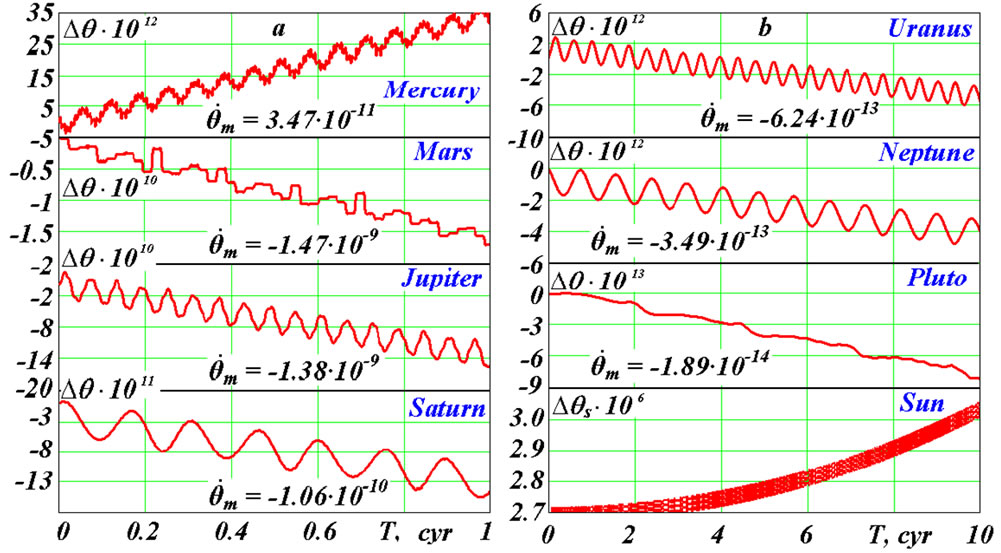
Figure 8. Nutation oscillations and trends of the Earth’s axis at separate action of the planets and the Sun as difference  for planets and as sliding average
  for the Sun. See captions on Figure 3.

Table 3. Periods of the Earth’s axis oscillations, their amplitudes and mean nutation rates at separate action of the Sun, the Moon and the planets: 1)* periods and amplitudes caused by approach in equatorial plane; sidereal half–cycles (TB·0.5) of the Earth, the Moon and the planets round the Sun are given after “/”; 2)** period and amplitude caused by precession of orbital plane of the Moon.
becomes complicated as the majority of authors do not submit these equations in a final kind. With the purpose of their approximate solution the differential equations of the 2nd order are simplified to equations of the first order (the Poisson equations). Additionally, different reference systems, different variables and different designations are used, and no one work known to us has the equations in a final form similar to (41), (42). P. Bretagnon et al. [9] gives the fullest kind of the differential equations from the latest works. At substitution in the equations of these authors the moment Jy = Jx, and angular velocity according to (40), terms, caused by the angular momentum, coincide with corresponding terms of our Equations (41) and (42). These authors express terms, caused by the torques, by Legendre polynomials, therefore they cannot be compared with our terms.
Our solution (40) for the Earth’s angular velocity  and kinematic terms of Equations (41) and (42), taking into account the signs of
  and
and , also coincide with the Equations (9.1.04) and kinematic terms of Equations (9.1.05) given by G. Duboshin [17], if to consider two typing errors in Equation (9.1.05). These typing errors in the subsequent Poisson Equation (9.1.06) are eliminated. By comparison of the equations, typing errors in other works are found out. This circumstance is an additional argument in necessity of the work on the derivation of the Earth’s rotational motion equations.
Our derivation of the torques coincides with a tradi- -tional derivation [15] up to expression (31) inclusively before the force function U. After that the values ri3 and (zi/ri) are usually represent in series on elements of elliptic motion on the basis of the theory of secular perturbations. So these results also are non-comparable to ours.
As a result it is possible to make the following conclusion. The terms of Equations (41) and (42), caused by the angular momentum, coincide with the equations of other researchers. The terms of the equation, caused by the torques, also coincide at identical stages of the derivation. The accepted way of derivation of the equations, the approach to their solution, the initial condition setting and the final kind of (41), (42) do not repeat the equations, known to us in the literature. Despite originality of these methods for the Earth’s rotational motion equations, they are typical in the mechanic and are traditionally used in its different areas.
In our solutions daily oscillations of the angles of precession  and nutation
  are received. P. Bretagnon et al. [9] carried out numerical integration for check of the analytical solutions. Differences between the numerical and analytical results, submitted in their work, have daily oscillations, i.e. numerical solutions of these authors also give daily oscillations. Daily frequencies of oscillations
  and
and  also exist in the observation data presented in the form of series [8].
Table 4 gives the comparison of the amplitudes and the periods of the Earth’s axis oscillations of the second and third types received by us (Sm) with the results of Bretagnon et al. [9] analytical solutions (Br). The mean precession and nutation rates, caused by the action of the Sun, the Moon and the planets, are compared here also. The amplitudes of oscillations  and
and , their period Т for the Sun and the mean precession speed
  coincide well. It is necessary to notice that the rate
 , according to Figure 8, changes nonlinearly, and its almost zero mean value during the initial moment against considerable semi-annual oscillations cannot be defined precisely. Due to this reason it is impossible to obtain the Moon’s rate
 .
.
The periods of oscillations Т of the angles, as we see from Table 4, well coincide for all the planets. Amplitudes of oscillations  and
and  are also well harmonized for the given planets from Jupiter to Neptune. Smaller conformity for the near planets is explained by difficult structure of oscillations
  and
and . In work [9] amplitudes are defined by representation of solutions as
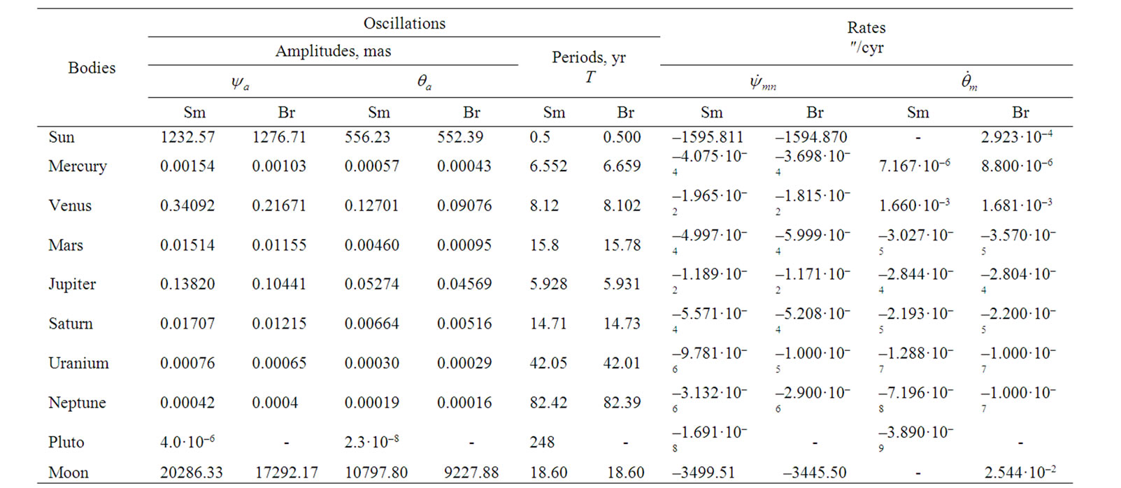
Table 4. Comparison numerically calculated (Sm) the Earth’s axis oscillations and mean rates of its motion with analytical results (Br) Bretagnon et al. (1997).
harmonious series; their main harmonics are given in Table 4. In our work actual amplitudes are defined by a sliding average method. These methods yield different results at difficult structure of oscillations.
The mean rates of change  and
and  at action of the planets, as we see from Table 4, are well correlated. Note, that exact coincidence of our and P. Bretagnon et al. [9] results is impossible, since there are difference in ways of parameters definition and in the initial data also. For example, at identical dynamical ellipticity Ed = EdS, our mean rate of precession for the action of the Moon is –3445.90, which practically coincides with P. Bretagnon et al. [9] result (–3445.50), see Table 4.
As the solutions of P. Bretagnon et al. [9] are normalized by the observation data, coincidence of our results with results of these authors testifies their confirmation by observation data. The coincidences of our results (given to Table 4) testify reliability of the obtained differential equations and their solutions. This coincidence testifies also the correctness of the initial data. The mathematical model of motion of the planets and the Moon, which gives their positions in process of numerical integration of Equations (41) and (42), proves to be true also. It is necessary to notice also that in [9] the Earth is considered as non-axisymmetrical, power function is estimated by potential of the surface distribution of gravity and geodetic precession is taken into account. All these additional influences give additives which are in limits of differences of our solutions from Bretagnon et al. [9].
8. Conclusions
1) The law of angular momentum change is analyzed and on its basis the differential equations of the Earth’s rotational motion for the gravitational action of the Solar system bodies is derived.
2) The algorithm and the program of numerical integration of obtained equations are developed.
3) The equations are integrated separately taking into account the action of the Sun, the planets and the Moon on the Earth over 10 kyr and results are analyzed.
a) The greatest action on the Earth rotation is from the Moon, then from the Sun, and from Venus among the planets.
b) The precession ψ, nutation θ and rotation φ angles change with identical periods controlled by the periodicity at which the bodies cross the Earth’s equatorial plane and approach the Earth, and by the precession of the orbital plane relative to equatorial plane.
c) The action of the Moon, the Sun and the planets has caused a clockwise precession of the Earth’s axis at an almost invariable mean rate.
d) For this time span, the nutation angle θ has increased under the action from the Sun, the Moon and the inner planets or decreased under the action from the outer planets.
4) The results are confirmed with other reported data and with observations.
9. Acknowledgements
A.E. Lutsky and A.O. Latsis from the Keldysh Institute of Applied Mathematics (Moscow) assisted in computation on an HVS-1000 supercomputer. Computation was also run on HVS-1000 and NKS-30T supercomputers of SB RAS Computing Center, (Novosibirsk) with the help of A.S. Alekseev, V.P. Kutov, N.V. Kuchin and V.D. Korneev. K.E. Sechenov took part in the study of the Earth’s rotation for the action of the Sun and the planets and K.S. Ivanov took part in the study of the Moon’s action. I express the gratitude to all aforementioned colleagues.
The study was supported by grants from the Governor of Tyumen Region (in 2003 and 2004) and was carried out as part of Integration Programs 13 (2004-2009) of the Presidium of the Russian Academy of Sciences.
10. References
[1] M. Milancovitch, “Mathematische Klimalhre und Astronomische Theorie der Klimaschwankungen,” Gebruder Borntraeger, Berlin, 1930.
[2] D. Brouwer and A. J. J. Van Woerkom, “The Secular Variation of the Orbital Elements of the Principal Planets,” Astronomical Papers, Vol. 13, 1950, pp. 81- 107.
[3] Sh. G. Sharaf and N. A. Budnikova, “O Vekovykh Izmeneniyakh Elementov Orbity Zemli, Vliyayschikh Na klimaty Geologicheskogo Proshlogo (The Secular Variation of the Orbital Elements of the Earth as a Control of Past Climates),” Bull. ITA AN SSSR, No. 11, 1967, pp. 231-261.
[4] A. Berger and M. F. Loutre, “Insolation Values for the Climate of the Last 10 million Years,” Quaternary Science Reviews, Vol. 10, No. 4, 1991, pp. 297-317. doi:10.1016/0277-3791(91)90033-Q
[5] J. Laskar, F. Joutel and F. Boudin, “Orbital, Precessional and Insolation Quantities for the Earth from –20 Myr to +10 Myr,” Astronomy and Astrophysics, Vol. 270, No. 1-2, 1993, pp. 522-533.
[6] V. P. Melnikov and J. J. Smulsky, “Astronomical Theory of Ice Ages: New Approximations, Solutions and Challenges,” Academic Publishing House, Novosibirsk, 2009.
[7] P.-S. Laplace, “Précis de l’histore de l’astronomie,” In: P.-S. Laplace, Ed., Ocuvres Complétes, Tome VI, Livre V, Gautier-Villars, Paris, 1878-1912, pp. 454-486.
[8] P. M. Mathews and P. Bretagnon, “Polar Motions Equivalent to High Frequency Nutations for a Nonrigid Earth with Anelastic Mantle,” Astronomy & Astrophysics, Vol. 400, No. 3, 2003, pp. 1113-1128.
[9] P. Bretagnon, P. Rocher and J. L. Simon, “Theory of the Rotation of the Rigid Earth,” Astronomy and Astrophysics, Vol. 319, 1997, pp. 305-317.
[10] T. R. Quinn, S. Tremaine and M. Duncan, “A Three Million Year Integration of the Earth’s Orbit,” Astronomical Journal, Vol. 101, 1991, pp. 2287-2305.
[11] P. Bretagnon and J. L. Simon, “Towards the Construction of a New Precession-Nutation Theory of Nonrigid Earth,” Celestial Mechanics and Dynamical Astronomy, Vol. 80, No. 3-4, 2001, pp. 177-184. doi:10.1023/A:1012265826581
[12] J. J. Smulsky, “The Theory of Interaction,” Publishing House of Novosibirsk University, Novosibirsk, 1999. (In Russian) http://www.ikz.ru/~smulski/TVfulA5_2.pdf
[13] J. J. Smulsky, “The Theory of Interaction,” Cultural Information Bank, Yekaterinburg, 2004. (In English) http://www.ikz.ru/~smulski/TVEnA5_2.pdf
[14] H. Lamb, “Dynamics,” Cambrige University Press, Cambrige, 1929.
[15] W. M. Smart, “Celestial Mechanics,” John Wiley, New York, 1961.
[16] S. Newcomb, “The Elements of the Four Inner Planets and the Fundamental Constants of Astronomy,” Government Printing Office, Washington, 1895.
[17] G. N. Duboshin, “Nebesnaya Mekhanica I Astrodinamica (Celestial Mechanics and Astrodynamics),” Nauka, Moskva, 1976.
[18] F. Roosbeek and V. Dehant, “RDAN97: An Analytical Development of Rigid Nutation Series Using the Torque Approach,” Celestial Mechanics and Dynamical Astronomy, Vol. 70, No. 4, 1998, pp. 215-253. doi:10.1023/A:1008350710849
[19] J. L. Simon, P. Bretagnon, J. Chapront, M. ChaprontTouzé, G. Francou and J. Laskar, “Numerical Expressions for Precession Formulae and Mean Elements for the Moon and Planets,” Astronomy and Astrophysics, Vol. 282, No. 2, 1994, pp. 663-683.
[20] J. J. Smulsky, “Osesimmetrichnaya Zadacha Vzaimideistviya N-tel (The Axisymmetrical Problem of Gravitational Interaction of N Bodies),” Matematicheskoe Modelirovanie, Vol. 15, No. 5, 2003, pp. 27-36. (In Russian) http://www.smul1.newmail.ru/Russian1/IntSunSyst/Osvnb4.doc
[21] J. J. Smulsky, “Matematicheskaya Model Solnechnoi Sistemy (A Mathematical model of the Solar System),” In: V. A. Bereznev, Ed., Teoreticheskie i Pricladnye Zadachi Nelineinogo Analiza, Vychislitelny Centr Imeni Dorodnitsyna, Moskva, 2007, pp. 119-139. (In Russian) http://www.ikz.ru/~smulski/Papers/MatMdSS5.pdf