Advances in Chemical Engineering and Science
Vol.3 No.4A(2013), Article ID:37261,9 pages DOI:10.4236/aces.2013.34A1002
Theoretical Evaluation of Two-Phase Flow in a Horizontal Duct with Leaks
1Department of Chemical Engineering, Center of Science and Technology, Federal University of Campina Grande (UFCG), Campina Grande, Brazil
2Department of Mechanical Engineering, Center of Science and Technology, Federal University of Campina Grande (UFCG), Campina Grande, Brazil
Email: morganamva@gmail.com, fariasn@deq.ufcg.edu.br, gilson@dem.ufcg.edu.br
Copyright © 2013 Morgana de Vasconcellos Araújo et al. This is an open access article distributed under the Creative Commons Attribution License, which permits unrestricted use, distribution, and reproduction in any medium, provided the original work is properly cited.
Received July 23, 2013; revised August 23, 2013; accepted September 4, 2013
Keywords: Two-Phase Flow; Numerical Simulation; Leakage; Pipeline
ABSTRACT
The transport of oil and its derivates are done, mostly, by pipeline. The time to detect leaks has to be short for preventing big disasters in the nature and decreasing losses for industries. The techniques available for leak detection vary from visual inspection to the use of computational techniques such as mathematical modeling. This paper aims to study the fluid dynamics of two-phase flow (water-oil) in the pipe with leakage. The equations of the mass and momentum conservation are numerically solved by using the ANSYS® CFX commercial code with the aid of a structured mesh of a horizontal pipe with three holes of leaks. The Eulerian-Eulerian model was adopted considering the oil as continuous phase and water as dispersed phase, and constant fluid properties. With profiles of pressure and volume fraction along the time in the pipe, the influence of leakage on the single-phase (oil) and two-phase (water-oil) was evaluated.
1. Introduction
The transportation of oil and its derivatives are mostly conducted through pipelines that connect production facilities, refineries and, in some situations, the consumer centers.
The materials used for making pipes come through technological improvements, where there is a significant use of materials based on special steel, lighter and stronger. However, despite these advances, there are still problems with leaks in pipelines generating great interest from the oil industry in view of the high costs incurred by financial services, potential risks and environmental costs.
Environmental disasters related to the oil spill in addition to degrading the environment, are responsible for spending millions of dollars in remediation.
In oil activities, particularly in transportation by pipelines, accidents have happened, causing financial and environmental losses.
There are currently a variety of techniques available for the detection of leaks, ranging from simple physical inspection by acoustic methods. Zhang [1] classified the detection methods into three categories: observation (perhaps the simplest and most ancient, is conducted through a visual inspection noting any ponding on the soil surface or anomalous growth of vegetation), direct detection (devices are used for the detection and location of leakage) and indirect detection (software is used based on mathematical models which allow to perform detection by means of data flow like pressure, temperature, mass flow rate, etc.).
The faster the identification of a leak in a pipeline, the faster valves are closed and the pumps will stop and, consequently, the greater the chances of avoiding a catastrophe are. However, in order to do the detection and precise identification of the position of a leak, it is necessary to know the behavior(s) of fluid(s) within the duct which allows determination of pressure drop between two points being evaluated.
According to Buiatti [2] the kind of leaks appearing in pipe networks can be divided into two classes:
1) Leak by “breaking” the tube—Occurs less frequently, but it is dangerous due to the amount of product spilled in the vicinity of the leak. However, these disruptions are easy to detect because they are accompanied by pressure losses and volumetric differences.
2) Leakage of small proportions—Small leaks around 5 liters per hour are difficult to detect due to their sizes and can cause large losses of products to get noticed. Maybe provided by corrosion, fatigue of the material that makes up the pipe or by failure is in welds. There are few methods capable of detecting leaks of this order.
The occurrence of a leak surely results in a disturbance in the behavior of pressure in the pipe and this disturbance can describe the location, the size and the altitude of the leak. A dynamic associated with the leak is propagated along the pipe from the point of the leak and with a variable speed, being perceived in different moments by sensors on the pipe. The location of the leak in the pipe is calculated from the time interval between the perceptions of the dynamic data from sensors coupled to the distance between the sensors. Azevedo [3] proposed the division of the temporal evolution of a leak in three steps:
1) Pre-Leak: it corresponds to the behavior of the flow in the pipe before the leak phenomenon and reflects the normal steady-flow conditions;
2) Transitional: it corresponds to the behavior of accommodation of the flow in the pipe from the initial leak until the moment of reaching a new steady state;
3) Post-Leak: it corresponds to the behavior of the flow in the pipe after the occurrence of a leak and the stabilization of the flow conditions, reflecting the flow stationary conditions on pipes with the presence of a leak Different works related to leakage in the pipe has been reported in the literature [4-8].
Agbakwuru [4] discusses about the challenges and technologies available for viewing and examination of leaks in pipelines located in the sea and under the conditions of poor visibility. It is proposed the use of Remotely Operated Vehicles with an optical eye as a tool to perform visual inspection of the pipeline and assist in the challenge of repairing the oil spill. The techniques used for pipelines submerged in water of poor visibility are based on tools used: hydrophone/Acoustic sensor, direct hydrocarbon leak detection, fluorescence. This author did a research about the oil/gas industry in the Nigeria Niger Delta Region. The causes of pipeline leaks were classified in operational, structural, unitended and intended damages. The Autor has shown the big values of leakes caused by sabotage in the Delta Region from the year 2005 to 2011. To reduce cost and improve effectiveness of systems of ducts in Delta Niger, it was proposed a combination of two methods of leak detection: the impressed alternating cycle current (IACC) for pipes with a small diameter (4 to 8 inches) and short length and the acoustic method for pipes with large diameter and long length.
Braga [5] evaluated air and water flow in a pipe with 1250 meters length. Coupled pipe flow is a data acquisition system, where this detection system has four pressure transducers connected to a computer equipped with an ADA converter board (Analog-digital-Analog). Three different types of flow regimes were studied: isolated bubbles of air without leak of the fluid, flow of a single air bubble in the presence of leak, and continuous flow air-water with leak. The experiments showed that the presence of air in the pipe generates reflections of waves (spring effect) that interferes with the detection of the leak. The author concluded that depending on the amount of air in the pipe, this can act as a damper of the shock wave, reducing the impact produced by leakage and thus, decreasing the sensitivity of the system.
The pressure transducers along the pipe convert pressure variations into variation of an electrical magnitude (voltage or current) to the PLC (programmable logic controller) which can work with this information. To drain compressed air Bezerra [6] built a pipe in PVC (polyvinyl chloride) with a diameter of 2.5 cm and a length of 5.56 meters. Two transducers were placed along the pipe and the transient pressure (pressure variation in the pipe with time) was measured simultaneously. The method detected the leak in the pipe, but we observed a difficulty in obtaining the location of the leak and this was explained by the fact that the two transients occur with a very small time difference, which was justified by the fact that the pipe had a short length. Bezerra [6] concluded that the program was successful in locating the leak which was necessary for the transducers installed at a distance farther than 12.24 meters from each other.
Garcia et al. [7] represented with the aid of commercial software COMSOL Multiphysics 4.0a®, a section of a pipe with 2 feet in length, 10 centimeters in diameter and a orifice leak of 4 mm in diameter. A cylindrical volume was linked perpendicularly to orifice surface to observe the leak jet. At the beginning, the pipe was completely filled with water at an absolute pressure of 101,325 Pa and the cylindrical volume had air at an absolute pressure of 0 Pa. Initially a leak test with a bench trial was held, where there was water inside the pipe and air was injected to study the flow behavior in the region of leakage. The numerical simulations were performed with the help of a mesh with 21.376 tetrahedral elements, with injections of air with a speed of 2 m/s and 10 m/s during a time interval of 1 second, considering laminar flow. This author analyzed the magnitude of the velocity profiles in a central plane of the section of duct and observed that in the region of the leak there was an increase in speed, and, in the simulation with the higher speed, the values in the leakage region reached 425.5 m/s featuring a supersonic behavior in this region.
Sousa et al. [8] simulated a rising flow of an isothermic water/oil two-phase mixture. The domain of flow is a vertical duct 8 meters long and a diameter of 15 cm, with an orifice leak of 6 mm located at 4 m of inlet section. The mesh was done on the domain and has 327,327 hexahedral elements. The simulation was performed in ANSYS CFX 11.0. The authors varied the volumetric fraction of oil in the inlet flow duct in amounts of 0.75 to 1 and it was noted that the smaller was the oil fraction, the major was the water fraction in the mixture and, consequently, the major was the mass flow through the orifice leak. The inlet velocities of mixture were varied and it was possible to realize that from 0.75 to 1.5 m/s the rate between the mass flow of leakage and total mass flow in the inlet section decreased with the increase of the velocity, but between 1.5 and 2 m/s the effect was the opposite due to inertial forces of flow being smaller than the forces caused by pressure drop from inlet to the leak. Complementing the authors’ conclusions, it is observed that the emergence of the leak causes a pressure drop which is directly proportional to the volume fraction of water in the mixture and the flow rate of the same.
In this context, the proposed research is to contribute to the study of leakage and help to understand the phenomenon involved via techniques of computational fluid dynamics. This work aims to study numerically the twophase flow (water-oil) in a horizontal tube in the presence of leakage.
2. Methodology
2.1. Study Domain
To study the influence of leak in the hydrodynamics of the oil-water two-phase flow in a horizontal pipe, was adopted a study domain. The representation of the computational domain was done with the aid of ICEM-CFD 12.1 with points, curves and surfaces (Figure 1). The study area consists of a horizontal pipe with 10 meters long and 20 inches in diameter. The tube contains two holes of 1.6 cm diameter at the points (x = 5 m, y = 0.1 m, z = 0 m) and (x = 7.5 m, y = 0.1 m, z = 0 m) and a third hole of 3 cm diameter at the point (x = 5 m, y = −0.1 m, z = 0 m).
The representative mesh of the pipe was generated using the block strategy, which a single block is initially

Figure 1. Geometry with the regions of leak.
created involving the area of study and then the block is subdivided into several others. This strategy allows greater control of mesh refinement in regions desirable. The mesh was refined on the geometry and contains approximately 327,000 control volumes as shown in Figure 2.
2.2. Mathematical Modeling
In the studied flows, both monophase (oil) and the twophase (water-oil) flows, they are based on the following considerations:
1) Transient and laminar flow;
2) The fluid is newtonian and incompressible and the physicochemical properties are constants;
3) Isothermal process;
4) There is no occurrence of chemical reactions;
5) It was considered the gravitational effect;
6) No transfer of mass and momentum at the interface water and oil phases;
7) The interfacial forces of no drag (forces of lift, wall lubrication, virtual mass, pressure and turbulent dispersion of solid) were neglected.
The equations that describe the flow was withdraw from CFX 12.1®.
The equation of mass conservation is:
 (1)
(1)
where the the greek subscript ![]() represents the involved phase in two-phase mixture of water/oil; f,
represents the involved phase in two-phase mixture of water/oil; f,  , and
, and  are respectively the volumetric fraction, density and velocity vector. For the phase
![]() , the velocity vector is given by
, the velocity vector is given by .
.
The equation of momentum is:

Figure 2. Representation of the mesh tube and the detail of section of (a) leaks at x = 5m; (b) leak at x = 7.5 m; (c) input; (d) output and (e) one of the leaks.
 (2)
(2)
where p is the pressure,  represents the external forces acting on the system per unit volume,
  describes the overall force per unit volume (interfacial drag forces).
The interfacial drag force is given by:
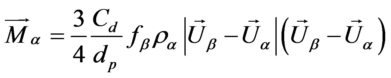 (3)
(3)
where dp is the particle diameter and Cd is the drag coefficient calculated using the Schiller-Neumann correlation, as follows:
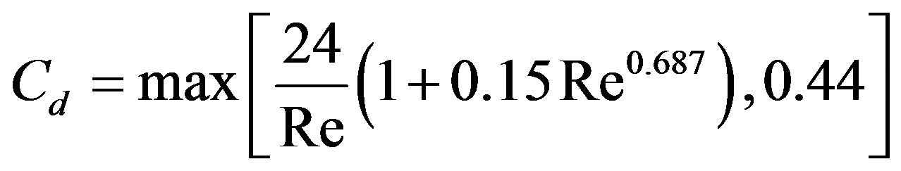 (4)
(4)
It was adopted the model of particle (Eulerian-Eulerian approaches) where oil behaves as a continuous fluid and water as spherical particles dispersed.
The simulations occurred in transient regimes and time steps were applied with 15 iterations each. In a period 0 to 0.01 second the flow time step used was 0.001 second; from 0.01 to 0.1 second the time step value increased to 0.01 second and after elapsed time 0.01 second the time step became 0.1 second.
The initial and boundary conditions are:
1) At the inlet:
a) The monophase flow has the characteristics:
i) Speed of oil-ux = 0.2 m/s;
ii) Entrance length: Le = 1.43 m.
b) For the two-phase flow (water-oil) we have:
i) The speed of the mix flow of water and oil-ux = 0.2 m/s;
ii) Volume fraction-foil (Table 1);
2) At the output: prescribed static pressure equal to 101,325 Pa;
3) At the wall:
a) No slip: ux = uy = uz = 0;
b) The smooth tube;
c) The static walls.
d) In the leak: average static pressure with value 101,325 Pa.
4) Pressure of reference: 0.0 Pa.
2.3. Physico-Chemical Properties
The properties of the fluids used in the present work, are shown in Table 2.
2.4. Case Studies
The simulations were performed to analyze the influence
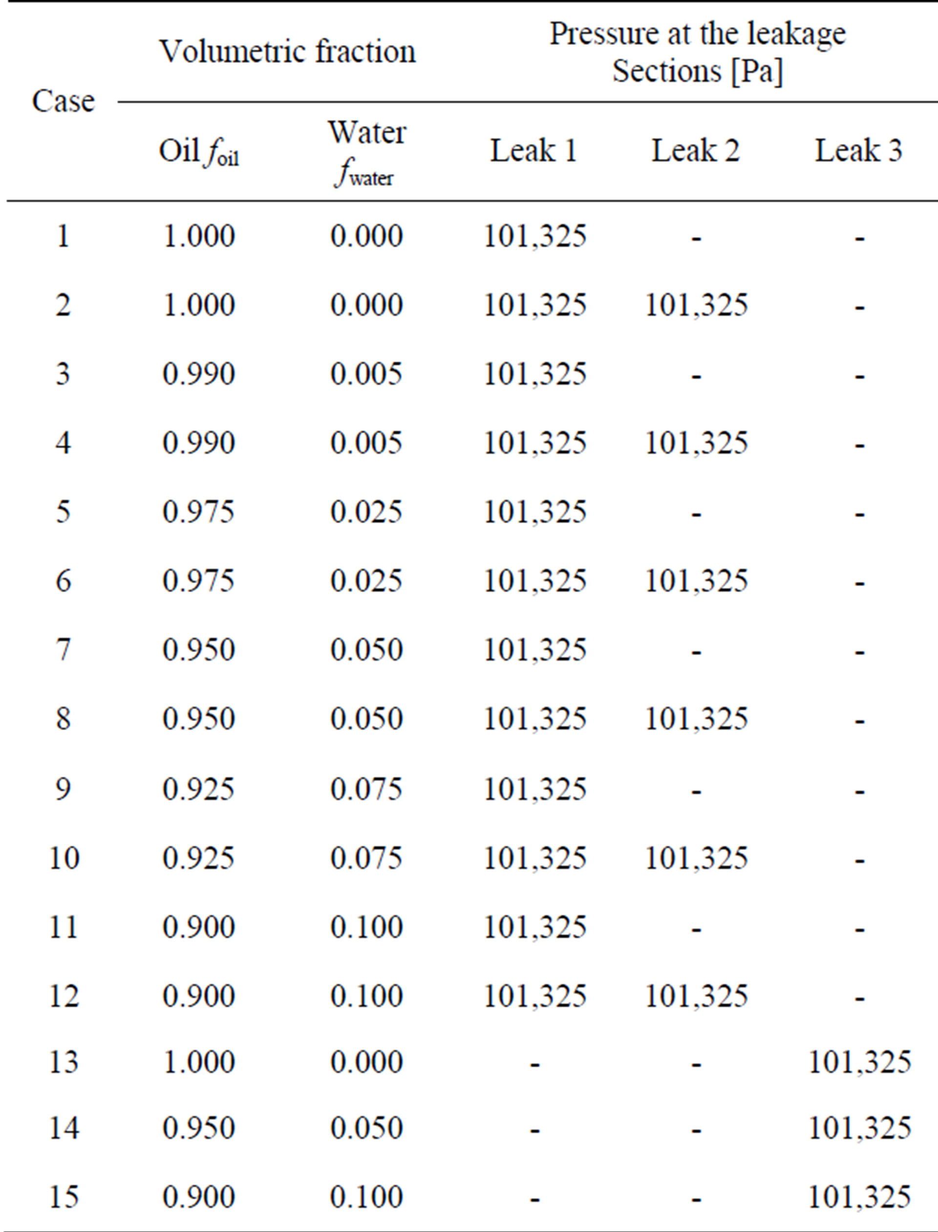
Table 1. Data used in the simulations.
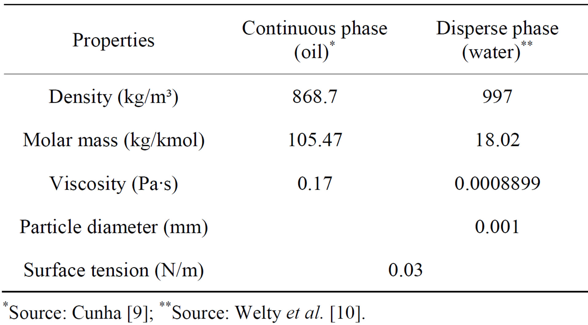
Table 2. Fluid properties.
*Source: Cunha [9]; **Source: Welty et al. [10].
of the oil volume fraction in the amount of oil leaked, as the disorder caused by the presence of two leaks in hydrodynamic flow. The influence of orifice size of leak in the monophase flow of oil and two-phase flow of oil and water were also studied. The constructed geometry can be maintained in its original position or undergo a 180˚ degrees rotation around the x axis, depending on each case, so that in all cases studied the opening of the leakage always occurs at the bottom of the pipe. The case studies are listed in Table 1. The simulations were investigated using computers with Quad-Core Intel Xeon Processor E5430 Dual 2.66GHz with 8GB of RAM.
The leakage in 5 m from the fluid inlet section (hole diameter = 1.6 cm) is called Leak 1, the leakage in 7.5 m from the fluid inlet section (hole diameter = 1.6 cm) is called Leak 2 and the leakage in 5 m from the fluid inlet section (hole diameter = 3.0 cm) is called Leak 3.
3. Results and Discussion
3.1. Fluid Volumetric Flow Rate Analysis
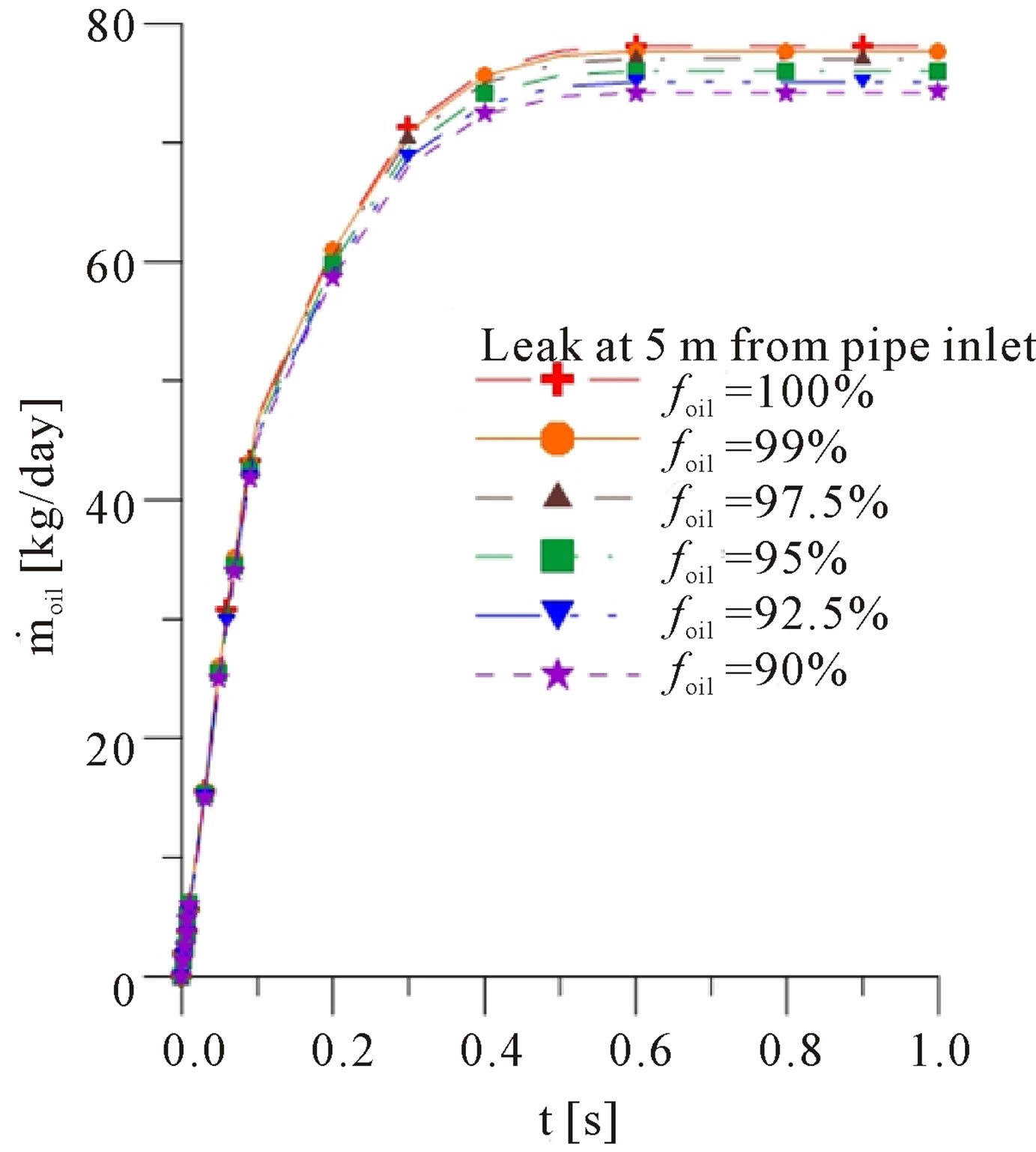
Figure 3 shows the evolution of the oil mass flow rate on the leak located at 5 m from inlet, with diameter of 1.6 cm, located in bottom side of pipe (Figure 1 rotated 180˚ around x axis). Figure 3(a) shows the evolution for cases where only the leak located at 5 m from inlet is activated (Cases 1, 3, 5, 7, 9 and 11) and the Figure 3(b) shows the same trend for the cases where the leaks at 5 m and at 7.5 m from inlet, with the same dimensions, are enabled (Cases 2, 4, 6, 8, 10 and 12). It is observed a similar behavior of the curves. With the decrease in volume fraction of oil entering the duct, it is observed a reduction of oil flow through the orifice leak. At the initial instants of the process, oil mass flow rate increase quickly until 0.4 s, when this time reaches the equilibrium condition (steadystate flow).
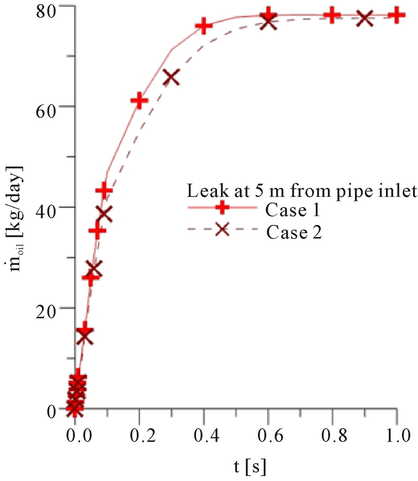
Figure 4 was done for continue the analysis of the oil mass flow rate at the hole cited before. It’s notable that the presence of the second leak disturbs the behavior of the flow, changing the oil mass flow rate on the first leak. The solid line corresponds to the oil mass flow rate for the cases when only the leak at 5 meters from the input section is activated. The dashed line corresponds to the oil mass flow rate in the same region, but when the first
 (a)
(a)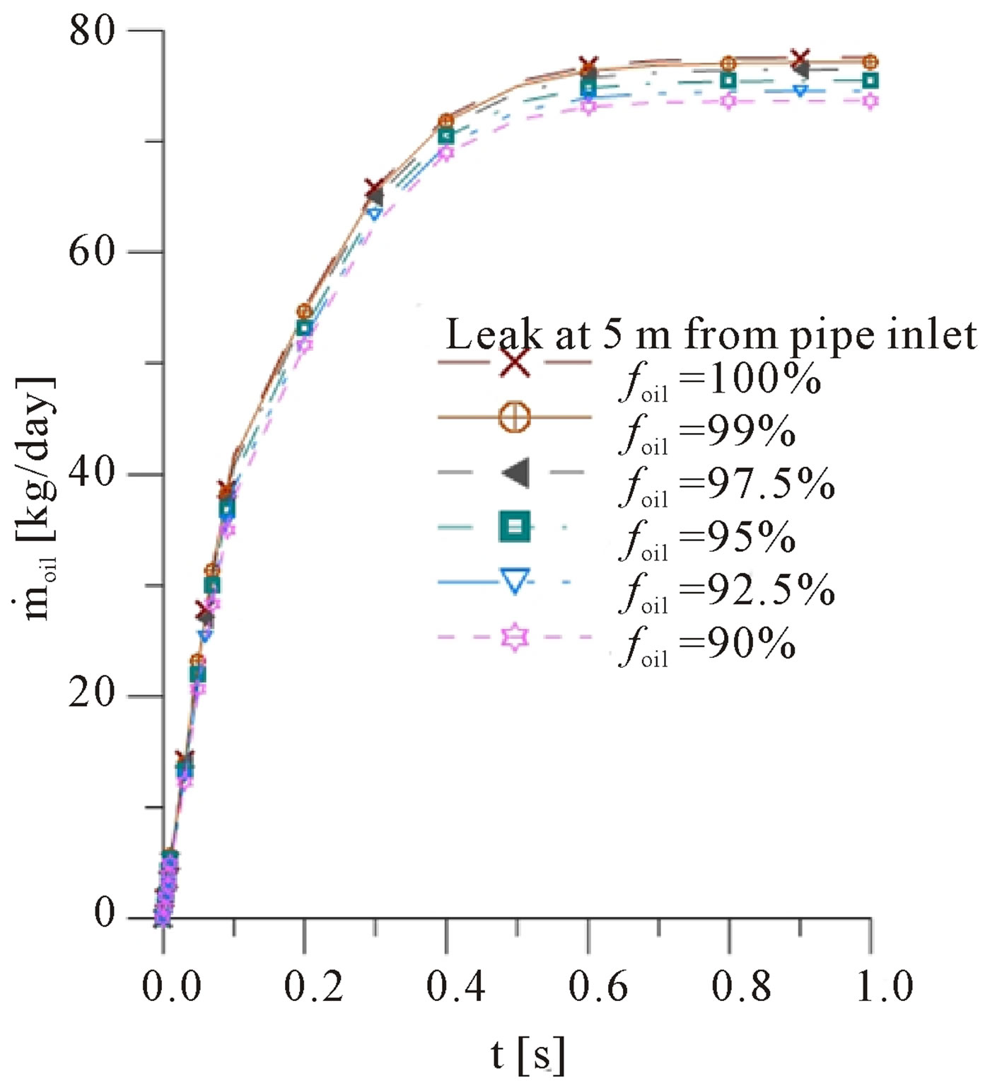 (b)
(b)
Figure 3. Oil mass flow in the orifice leak with diameter of 1.6 cm located at 5 m from the inlet versus time for different oil volumetric fractions injected into the pipe (a) Cases 1, 3, 5, 7, 9 and 11 and (b) Cases 2, 4, 6, 8, 10 and 12.
 (a)
(a) (b)
(b)
Figure 4. Oil mass flow rate in the orifice leak with diameter of 1.6 cm located at 5 m from the inlet versus time for different oil volumetric fractions injected into the pipe (a) Cases 1 and 2 and (b) Cases 11 and 12.
and second leaks are activated simultaneously. Comparing the two curves mentioned above, for the Cases 1 and 2 (Figure 4(a)), we see that the flow described by the continuous curve is stabilized higher and faster than the represented by the dashed curve flow. The same behavior is observed for the Cases 11 and 12 (Figure 4(b)).
For a better view of the graph (Figures 5 and 10), we adopted the dimensionless time as follows:
 (5)
(5)
were t is the time and ttotal is the total time of simulation. For the cases 01, 07 e 11 were adopted the total time of 1 second. For the cases 13, 14 and 15 the value is 1.8 s.
To analyse the effect of the orifice leak diameter on the oil mass flow rate, the cases 1, 7, 9, 13-15 are studied (Figure 5). To study the cases 13-15, where the leak is located in the bottom side of the pipe, the original position is maintained like the Figure 1 shows, i.e., the pipe is not rotated.
By increasing the diameter of the leak, it is observed that there is an increase in the oil mass flow rate in the leak, the continuous curve of Figure 5(a) is equivalent to the oil mass flow in Case 1, where the leak with a diameter of 1.6 cm and located at 5 meters from the input section is activated. The dashed curve refers to the oil mass flow rate in Case 13 where the leak with a diameter of 3.0 cm and located at 5 meters from the input section is activated. It is easily understood that the volumetric flow in the orifice with a diameter of 3.0 cm (dashed curve) is higher than for an orifice with a diameter of 1.6 cm (continuous curve). It is also interesting to note that by increasing the diameter of the orifice, more time is necessary to the oil mass flow rate to achieve the equilibrium condition. The same behavior is observed for Cases 7 and 14 (Figure 5(b)) and the Cases 11 and 15 (Figure 5(c)).
Figure 6 illustrates the result of the total mass flow rate in leakage as a function of oil volumetric fraction at the entrance of pipe, after 1 second of flow for leak with
 (a)
(a) (b)
(b)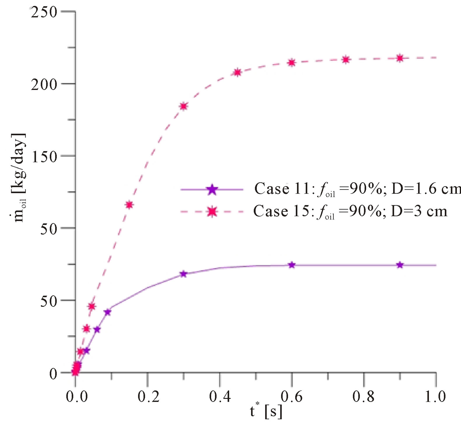 (c)
(c)
Figure 5. Oil mass flow rate in the leak versus dimensionless time for the leaks with different diameters.
a diameter of 1.6 cm and after 2 seconds of flow for leak with a diameter of 3.0 cm. It’s possible to see that the smaller oil volumetric fraction in the mixture, the higher is the total mass flow rate leaving the orifice, which can be attributed to a reduction in viscosity of the mixture. As expected, the bigger the orifice leak the greater the loss of the fluids.
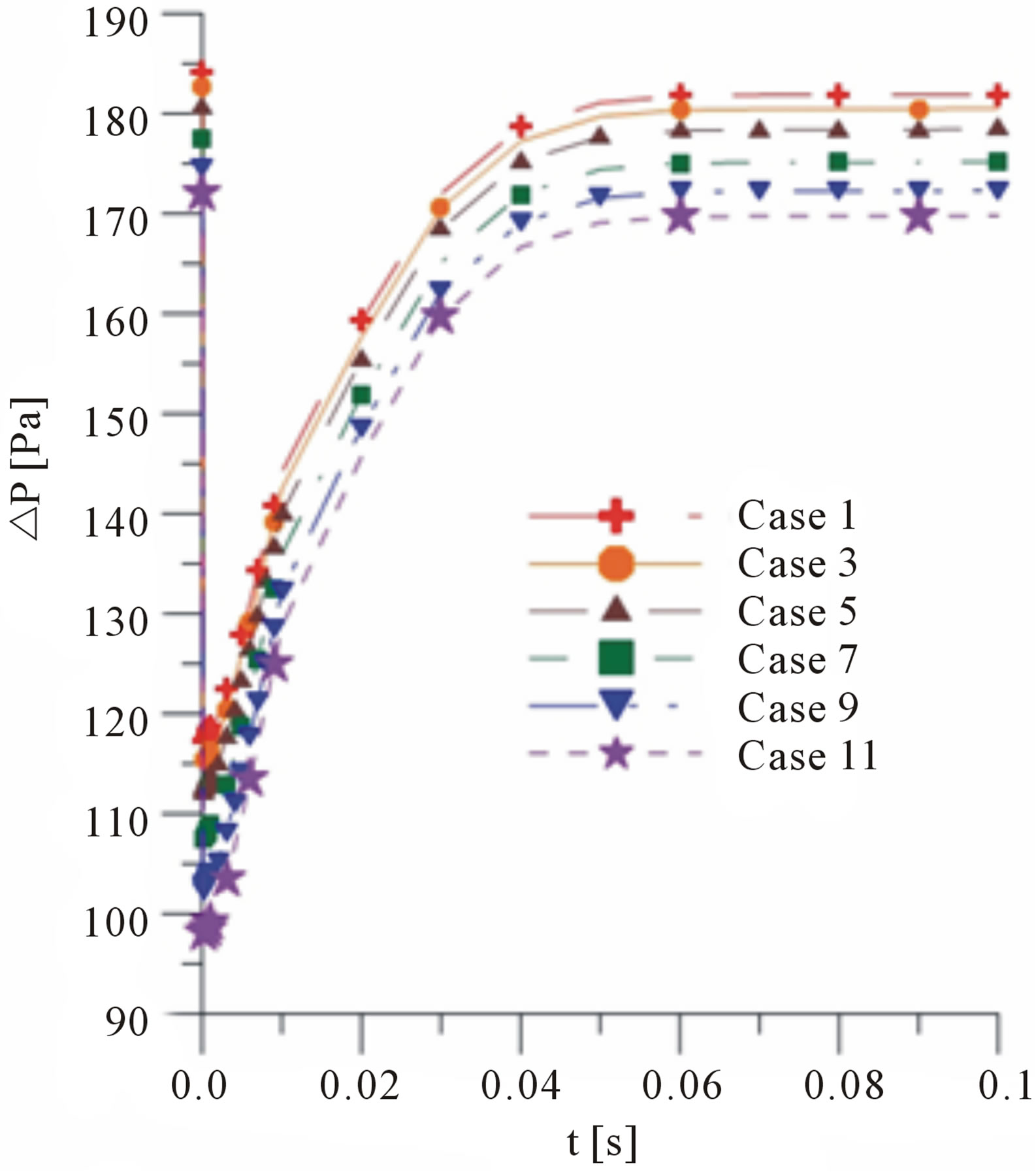
3.2. Pressure Drop Analysis
Figure 7(a) shows the evolution of the pressure drop between the entrance and the exit of the pipe as a function of time for different feeds of oil volume flow fractions when one leak is active (Cases 1, 3, 5, 7, 9 and 11). The similar behavior is observed, but with different magnitudes, for each value of the oil volumetric fraction and after 0.6 s of leaking there is a stabilization of the behavior of pressure. One fast drop in the pressure is verified at the initial instants of the flow due to presence of the leak.
The same behavior pressure drop between the inlet and outlet section is observed for cases where there are two active leaks, Figure 7(b) (Cases 2, 4, 6, 8, 10 and 12). However it is observed that the stabilization of the behavior of pressure occurs only after 0.7 s leak started. This behavior is explained by the fact two leaks in a same pipe cause a greater change as compared with the same pipe containing only one leak.
In order to observe the behavior of pressure along the duct, taken up average pressure values in different planes yz distributed along the duct (0, 1, 2, 3, 4, 4.5, 5, 5.5, 6, 7,
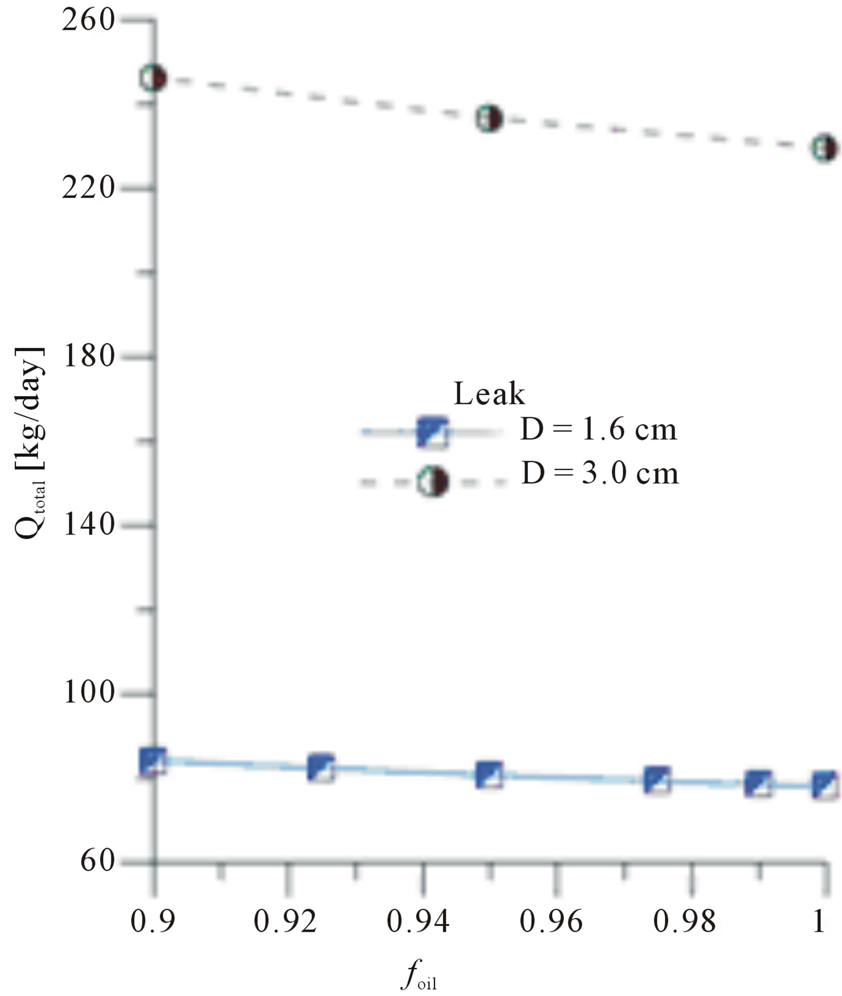
Figure 6. Oil-water mixture mass flow rate in the leak as a function of the oil volumetric fraction at the pipe inlet for leak with different diameters.
 (a)
(a) (b)
(b)
Figure 7. Pressure drop between the inlet and outlet sections of the pipe as a function of time and with presence of leakage (a) Cases 1, 3, 5, 7, 9 and 11 and (b) Cases 2, 4, 6, 8, 10 and 12.
7.5, 8, 9 and 10 m). With these average pressures were traced curves represented in Figure 8 for Cases 1, 3, 5, 7, 9 and 11 and Figure 9 for the cases 2, 4, 6, 8, 10 and 12 which shows the behavior of pressure along the duct. These curves were taken at the beginning of the leak (t = 0.001 s), t = 0.05 s, t = 0.1 s, t = 0.3 s and at the time that the behavior of the flow has been stabilized (t = 1 s). In all cases, the behavior change in pressure before and after the leak can be observed clearly.
By activating the leaks of 1.6 cm and 3 cm diameter, it is expected that they disturb the behavior of the pressure
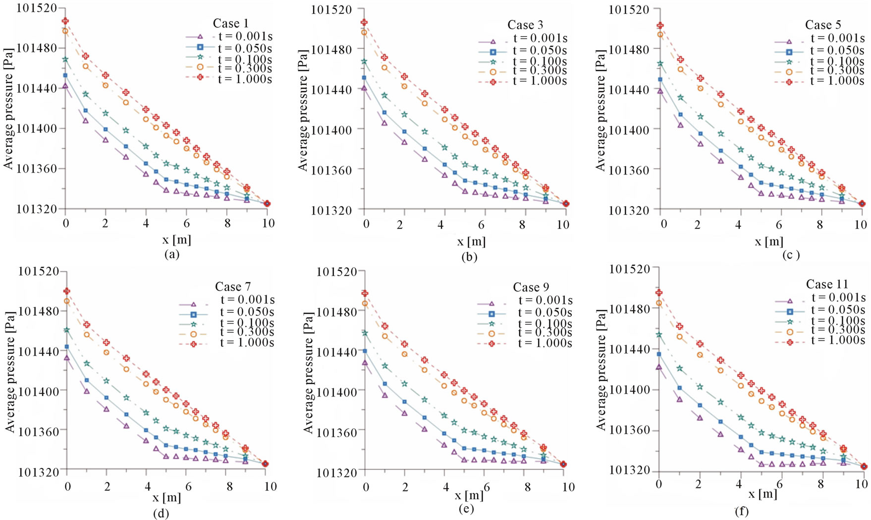
Figure 8. Average pressure along the duct at different flow time for the cases with only one leak.
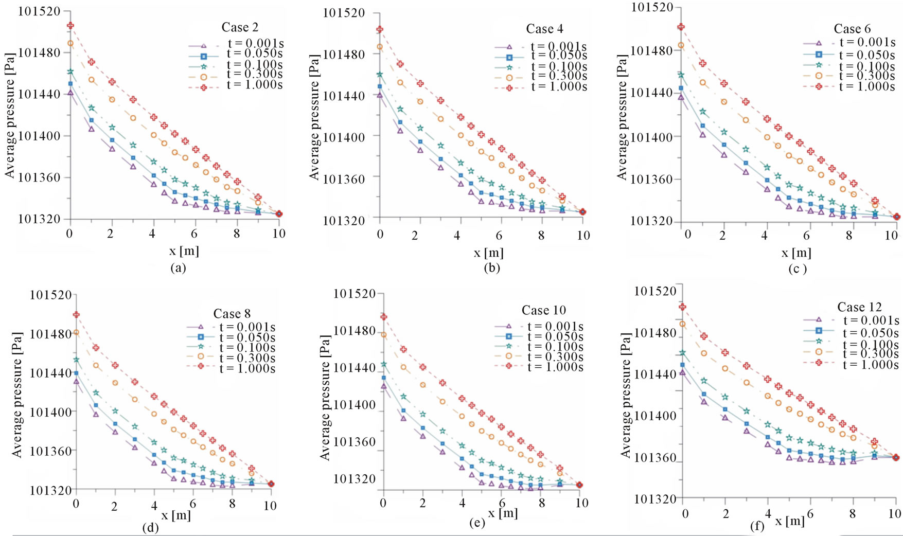
Figure 9. Average pressure along the duct at different flow time for the cases with two leaks.
in the duct. The results have proven that after a certain period of time the pressure in the duct turn back to stabilize. Figure 10 (oil monophase flow) shows that by varying the diameter of the leak, the pressure stabilization period also varies. The greater the leakage, the greater will be the disturbance, and therefore the time
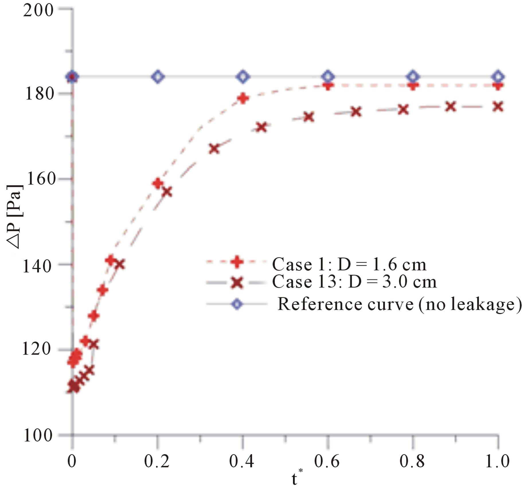
Figure 10. Average pressure drop between the inlet and outlet sections as a function of dimensionless time in the presence of leakage (Cases 1 and 13) and in the absence of leakage (reference curve).
taken to stabilize the pressure in a new value.
4. Conclusions
With the results of numerical simulation of single-phase flow (oil) and two-phase flow (water-oil) in pipes, it can be concluded that:
1) The proposed mathematical model was able to predict the leak in a horizontal pipe, evaluating the effect of the position, sizes and numbers of the leak on the fluid dynamic behavior of the mono and two-phase flows;
2) The volume fraction of oil in two-phase mixture injected into the duct affected the amount of oil leaked;
3) The presence of a second leak on downstream of the initial leakage on duct affected the oil flow of the first one, which became established with a lower flow rate compared to the situation where the first leak occured alone;
4) By increasing the diameter of the leak orifice, the greater the volume of fluid leaving the orifice was;
5) There was a slight variation of the pressure values before and after the leak and this varied depending on the fluid composition in the flow;
The time required for the pressure reaches stability after the leak depending on the size and locations of the leak in the pipe.
5. Acknowledgements
The authors would like to express their thanks to Capes, CNPq, FINEP, PETROBRAS, ANP/UFCG/PRH-25 and RPCMOD for supporting this work, and also grateful to the authors of the references cited in this paper that helped in the improvement of quality.
REFERENCES
- J. Zhang, “Designing a Cost Effective and Reliable Pipeline Leak Detection System,” Pipeline Reliability Conference, Houston, 19-22 November 1996, 11 Pages.
- C. M. Buiatti, “Monitoring of Tubes by Computational Thecniques On-Line,” Dissertation, Department of Chemical Engineering, State University of Campinas, Campinas, 1995.
- F. M. de Azevedo, “Proposal of Algorithm for Leak Detection in Pipelines Using Frequencial Analysis of Signals Pressure,” Dissertation, Federal University of Rio Grande do Norte, Natal, 2009.
- J. Agbakwuru, “Pipeline Potential Leak Detection Technologies: Assessment and Perspective in the Nigeria Niger Delta Region,” Journal of Environmental Protection, Vol. 2, No. 8, 2011, pp. 1055-1061. http://dx.doi.org/10.4236/jep.2011.28121
- C. F. Braga, “Leak Detection by Computer ‘On-Line’ in Tubes Transporting Mixture Gás-Liquid,” Master Dissertation, Department of Chemical Engineering, State University of Campinas, Campinas, 2001.
- B. A. F. Bezerra, “Leak Detection in Gas Pipelines by the Method of Transient Pressure Using CLP and Sensors,” Monograph (Conclusion of Specialization Course), Federal University of Pernambuco, Recife, 2008.
- F. M. Garcia, J. Giaretton, M. B. Quadri and A. Bolzan, “Fluidodynamic Simulation of Leaking Water in a Section of Duct for Applications in Oil & Gas Industry,” Proceedings of the 6th Brazilian Congress of Research and Development in Oil and Gas, Florianópolis, 9-13 October 2011, pp. 1-8.
- J. V. N. de Sousa, A. G. B. de Lima and S. R. de Farias Neto, “Numerical Analysis of Heavy Oil-Water Flow and Leak Detection in Vertical Pipeline,” Advances in Chemical Engineering and Science, Vol. 3, No. 1, 2013, pp. 9-15. http://dx.doi.org/10.4236/aces.2013.31002
- A. L. Cunha, “Advanced Non-Isothermal Recovery of Heavy Oil in Petroleum Reservoirs by Numerical Simulation,” Master Dissertation, Department of Chemical Engineering, Federal University of Campina Grande, Campina Grande, 2010.
- J. R. Welty, C. E. Wicks and R. Wilson, “Fundamentals of Momentum, Heat, and Mass Transfer,” 3th Edition, John Wiley & Sons, Hoboken, 1984.