Advances in Chemical Engineering and Science
Vol.3 No.1(2013), Article ID:26466,7 pages DOI:10.4236/aces.2013.31002
Numerical Analysis of Heavy Oil-Water Flow and Leak Detection in Vertical Pipeline
1Department of Mechanical Engineering, Center of Sciences and Technology, Federal University of Campina Grande, Campina Grande, Brazil
2Department of Chemical Engineering, Technology Center, Federal University of Alagoas, Maceió, Brazil
3Department of Chemical Engineering, Center of Sciences and Technology, Federal University of Campina Grande, Campina Grande, Brazil
Email: *joao.vns@hotmail.com
Received September 3, 2012; revised October 5, 2012; accepted October 14, 2012
Keywords: Heavy Oil; Multiphase Flow; Leakage; Numerical Simulation
ABSTRACT
Pipeline is a conventional, efficient and economic way for oil transportations. The use of a good system for detecting and locating leaks in pipeline contribute significantly to operational safety and cost saving in petroleum industry. This paper aims to study the heavy oil-water flow in vertical ducts including leakage. A transient numerical analysis, using the ANSYS-CFX® 11.0 commercial software is performed. The mathematical modeling considers the effect of drag and gravitational forces between the phases and turbulent flow. Mass flow rate of the phases in the leaking orifice, the pressure drop as a function of the time and the velocity distributions are presented and discussed. We can conclude that volumetric fraction of phases and fluid mixture velocity affect pressure drop and mass flow rate at the leak hole.
1. Introduction
The activity of oil production is subject to high risks. Even the petroleum industry running preventive measures, there is always the possibility of failure, making the industrial plants susceptible to operational accidents with loss of fluid to environment, causing great ecological, social and economic damages, with delay in oil production. A proper supervisory system must be capable of detecting leaks in oil installations, enabling immediate action to reduce the impacts of accidents and contributing significantly to operational safety. The simultaneous flow of two immiscible liquids in vertical pipes is encountered in different industrials processes and particularly in the petroleum industry [1].
Because of importance, many authors have focused their researches in methods of leak detection in pipes on oil production and transport [2-4].
However, in different applications, including oil transportation, accurate locations of the leaks is still very difficult. In present day various leak detection techniques based in the negative pressure wave, acoustic sensors, satellite surveillance, mass and volume balance, analytical model-based method, among others, has been applied. All these methods are based in process variables such as pressure, mass and volumetric flow rates and temperature [5].
According to Dong et al. [6], the negative pressure method, which supplies high leak sensitivity and availability, is a relatively better method among them. Unfortunately this method has a high possibility of false alarm if there are some strong raises in the pressure measurement records or if the leak is small (0.5% of nominal flow) [4,5].
Thus, this paper aims to numerically study the hydrodynamic of heavy oil-water flow in a vertical pipe having a small leak, which is much more difficult to detect by conventional systems [7]. The interest in heavy oil is in fact that recent studies indicate that in 2025 this kind of oil will be the main source of fossil energy in the world [8].
2. Methodology
2.1. The Geometry and Grid
The study domain (Figure 1) consists of a vertical pipe with 800 cm (8 m) of length, with a constant circular section 15 cm diameter. To simulate the leakage, the pipe has a circular hole, with 0.6 cm diameter, located at the midpoint of the length of pipe.
Figure 2 illustrates the mesh representing the study domain, which was built with the support of ICEMCFD® 11.0 software. This structured mesh was obtained after various refinements, and it has 327,327 hexahedral elements.
2.2. Mathematical Modeling
To investigate the multiphase flow of heavy oil-water in vertical pipes leaking, it was considered three-dimensional, transient and isothermal flow, non-homogeneous model for the fluid mixture (particle model) and homogeneous model for turbulence (k-ε model). The homogeneous model considers a single field for both phases, while in the non-homogeneous model is considered a specific field for each phase [9].
On the mathematical modeling, the index α represent the continuous phase (oil) and the index β represent the
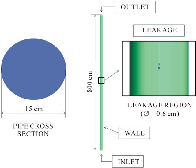
Figure 1. Considered pipe layout.
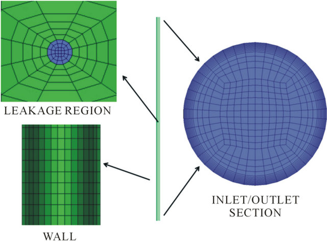
Figure 2. Studied pipe, showing different regions of the mesh.
dispersed phase (water). The dispersed water phase is modeled as spherical particles.
The general equations used in this work are:
• Continuity Equations,
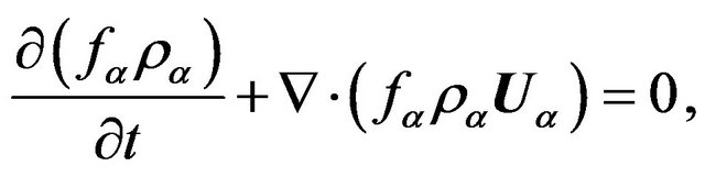 (1)
(1)
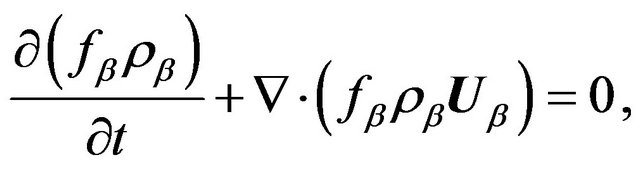 (2)
(2)
where f is the volume fraction, ρ is the density and  is the velocity vector, each corresponding to a given phase;
• Momentum Equations,
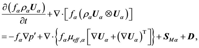 (3)
(3)
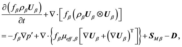 (4)
(4)
where p' is the modified pressure, μeff, is the effective viscosity, SM is the momentum sources due to external body forces (when gravitational forces are includes) and D is the drag force between the phases, that is modeled by the equation
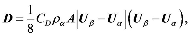 (5)
(5)
where CD is the drag coefficient and A is the interfacial area density. For Re < 1000, the drag coefficient is modeled by Schiller-Naumann model,
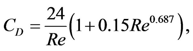 (6)
(6)
and for Re ≥ 1000, the drag coefficient is considered 0.44, where Re represents the particle Reynolds number, modeled by
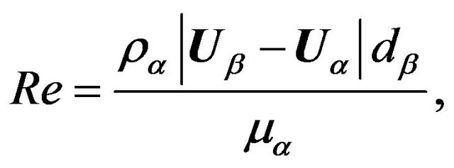 (7)
(7)
where dβ is the diameter of spherical particles (3 mm). The interfacial area density, A, is modeled by the equation
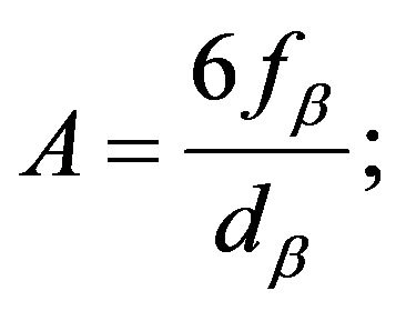 (8)
(8)
• Kinetic Energy Equation,
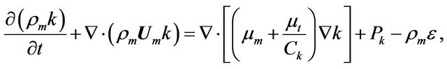 (9)
(9)
where ρm is the density, k is the kinetic energy,  is the velocity vector, μm is the viscosity, μt is the turbulent viscosity, Pk is the turbulence production and ε is the turbulence eddy dissipation, each corresponding to a mixture;
• Turbulence Eddy Dissipation Equation,
 (10)
(10)
where Ck = 1.0, Cε1 = 1.3, Cε2 = 1.44 and Cε3 = 1.92. In the k-ε model the parameters as follows
 (11)
(11)
 (12)
(12)
 (13)
(13)
 (14)
(14)
 (15)
(15)
 (16)
(16)
 (17)
(17)
 (18)
(18)
where pdin is the dynamic pressure, μα/μβ is the viscosity of phase and Cμ = 0.09. The dynamic pressure is calculated by the equation
 (19)
(19)
In multiphase flow, the total pressure acting in the phases, ptot, is modeled by
 (20)
(20)
where pst is a term correspondent to the static pressure.
2.3. Initial and Boundary Conditions and Fluids Properties
Initially (at time t = 0), the leak in the pipe does not exist, and the multiphase flow occurs in steady state condition. When t > 0 the leak appears abruptly in the pipeline. Tables 1 and 2 shows the initial and boundary conditions used in the simulations.
Simulations were performed with the following situations:
1) Oil volume fraction at the inlet, fo, ranging from 0.75 to 1.00 (step 0.05) and the water volume fraction at
Table 1. Boundary conditions for t = 0.
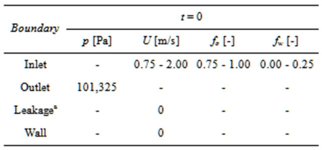
aImpermeable.
Table 2. Boundary conditions for t > 0.
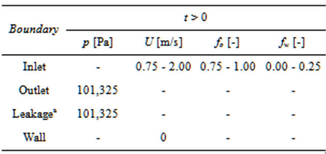
aOpening.
the inlet, fw, corresponds to the remaining fraction, with the velocity mixture at the inlet, U, fixed in 1.00 m/s;
2) Mixture velocity, U, ranging from 0.75 to 2.00 m/s (step 0.25), with the water volume fraction, fw, and oil volume fraction, fo, fixed in 0.15 and 0.85, respectively.
The adopted properties of the fluids are showed in Table 3.
Table 4 shows the considerations adopted for the numerical solver.
3. Results and Discussion
The simulations were performed on a Intel® Core 2 Quad 2.4 GHz, 4 GB RAM and 1 Tb physical memory (HD) computer. The solving time of the studied cases ranged from 10 to 11 hours.
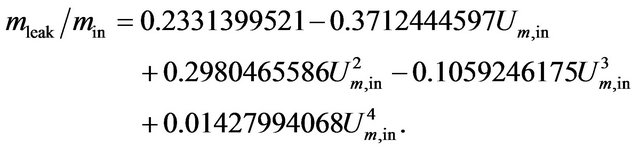
Figure 3 shows the total mass flow rate relationships on the leakage, mleak/min, as a function of oil volume fraction at the inlet section, fo,in, to post-leak system. We can see that the smaller the oil volume fraction, consequently, greater the water volume fraction in the mixture, thus we have a large amount of fluids exiting in the leak. This behavior is explained by the reduction of the viscosity of the fluid mixture, proportional to the water holdup contained in it. Figure 4 shows the total and oil mass flow rates in the leak, mleak, as a function of the oil volume fraction at the inlet section of pipe, to post-leak system. Note that the amount of water and oil mass flow rate in leak is proportional to the holdup of phases present in the mixture. Equations (21)-(23) were obtained by fitting the bared on the numerical data.
Table 3. Fluids properties.
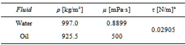
aτ is the oil-water surface tension.
Table 4. Numerical simulation characteristics.
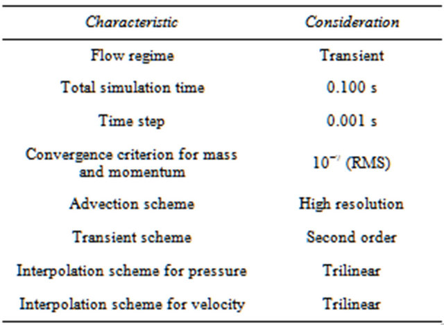
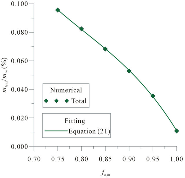
Figure 3. Total mass flow rate relationship in the leakage as a function of the oil volume fraction at the pipe inlet (U = 1.00 m/s).
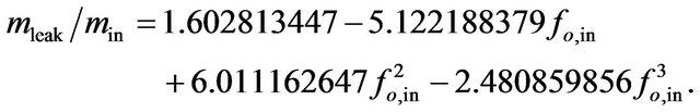 (21)
(21)
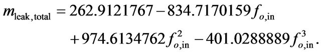 (22)
(22)
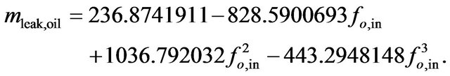 (23)
(23)
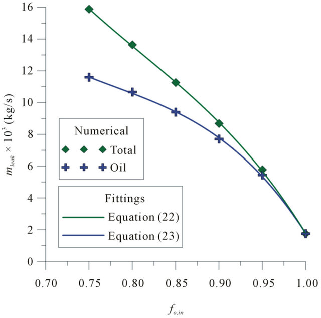
Figure 4. Total and oil mass flow rates in the leakage as a function of the oil volume fraction at the pipe inlet (U = 1.00 m/s).
Figure 5 shows the total mass flow rate relationships in leakage, mleak/min, as a function of the fluid mixture velocity at the inlet, Um,in, to post-leak system. It is noted that with increasing velocity, there is a reduction in the total mass flow rate through in the leaking. However, there is a reversal point (Um,in = 1.50 m/s), where by increasing the velocity of flow, we have an increased total mass flow rate in the leaking. This reversal point would be the point where the inertial forces of the flow becomes less than the forces caused by pressure differential between the inside and outside of the pipeline leaking (pressure gradients). Figure 6 shows the mass flow rate in the leak, mleak, as a function of the mixture velocity at the inlet, to post-leak. It is visible that increasing the mixture velocity at the inlet, the oil mass flow in the leaking increase, and the water mass flow is practically constant. Equations (24)-(26) were obtained by fitting the bared on the numerical data.
 (24)
(24)
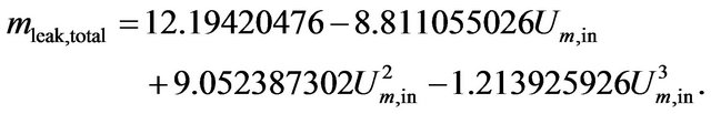 (25)
(25)
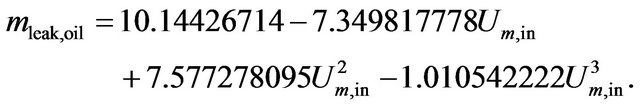 (26)
(26)
Table 5 shows the determination coefficients, R2, obtained in the fittings correspondents to Equations (21) to
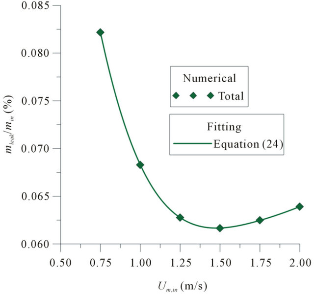
Figure 5. Total mass flow rate relationship in the leakage as a function of the fluid mixture velocity at the pipe inlet (fo,in = 0.85).
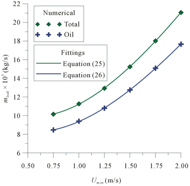
Figure 6. Total and oil mass flow rates in the leakage as a function of the fluid mixture velocity at the pipe inlet (fo,in = 0.85).
(26). These equations were obtained by the method of the least squares.
Figure 7 shows the oil velocity vectors at the leakage section, for some oil holdups in the mixture at the pipe inlet (fo,in = 0.80, 0.90 and 1.00). Note that by reducing the oil holdup, and thus, increasing the water holdup, there is a greater spread in the leakage, with a larger angle, taking as reference to the longitudinal direction of the pipe.
Figure 8 shows the velocity vectors at the leakage section, for some fluid mixture velocities at the pipe inlet
Table 5. Determination coefficients in the fittings.
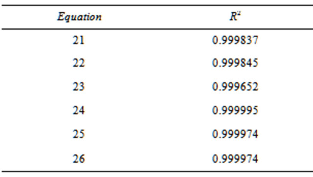
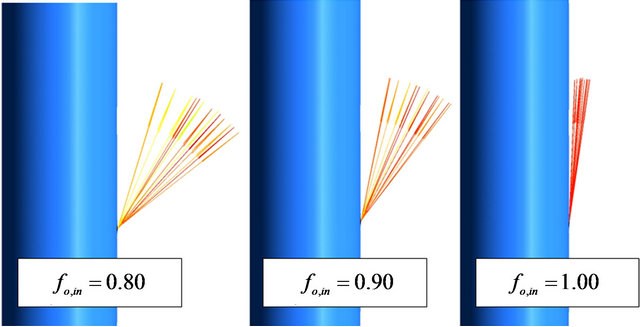
Figure 7. Velocity vectors at the leakage section, for some oil volume fractions in the mixture at the pipe inlet (Um,in = 1.00 m/s).
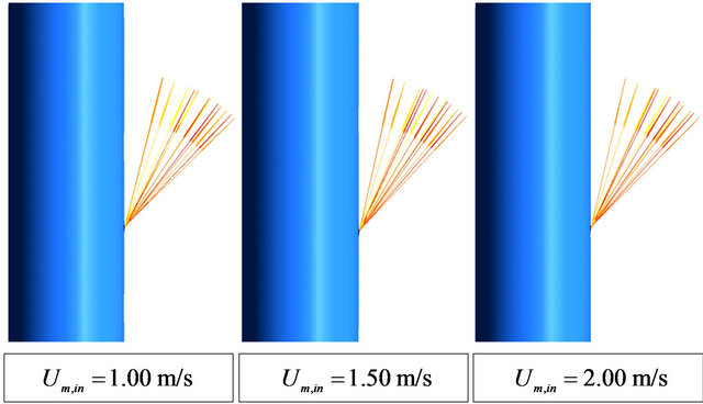
Figure 8. Velocity vectors at the leakage section, for some fluid mixture velocities at the pipe inlet (fo,in = 0.85).
(Um,in = 1.00, 1.50 and 2.00 m/s). It is visible the small influence of the velocity in the leak spread and angle.
Figure 9 shows the total pressure drop, Δptot, as a function of the time, t, for different oil volume fractions at the inlet, for a pipe section of 4 m length, where the leak is in the midpoint of this section. In all cases, it is visible reduction in the pressure drop at the initial instants of the leakage. The transient period is short (less than 0.03 s), as expected, due to low mass flow rate through out the leak hole. Reduction in the pressure drop is greater with the increase of the water holdup in the mixture. After the flow reaches a new steady state (t > 0.025 s), the pressure drop reach the same level before the leakage. This level is greater for the cases where the
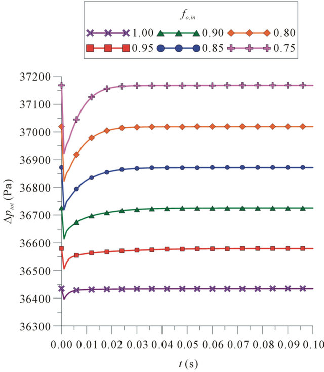
Figure 9. Pressure drop as a function of the time, for different oil volume fractions in the mixture at the pipe inlet (Um,in = 1.00 m/s).
water volume fraction in the mixture is greater, since the water has a density higher than the oil, increasing the static pressure drop portion, which is the most representative portion of the total pressure drop.
Figure 10 shows pressure drop as a function of the time, for different mixture velocities at the inlet, for a pipe section of 4 m length, where the leakage is located in the midpoint of this section. Similarly, it is visible the reduction in the pressure drop in the initial instants of the leakage. The transient period is too short, being less than 0.025 s. The higher pressure drop in transient state is obtained as the mixture velocity at the inlet is increased.
Figures 11 and 12 show, respectively, the total pressure and the oil velocity fields near the leakage section (in the transversal plan), for a case with the mixture velocity in the inlet 1.00 m/s and the oil and water volume fractions are 0.85 and 0.15, respectively. We can see that the leakage region is one zone of low pressure and high velocity. This behavior was found in all cases analyzed in this paper.
4. Conclusions
In this paper the hydrodynamic of two-phase flow in vertical pipe with a leakage is discussed. The study is related to heavy oil-water flow in the turbulent regime by using the ANSYS-CFX® 11.0 commercial software.
The simulations revealed the difficulty of detecting small leaks (less than 1% of the total mass flow rate
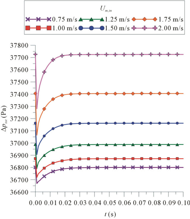
Figure 10. Pressure drop as a function of the time, for different mixture velocities at the pipe inlet (fo,in = 0.85).
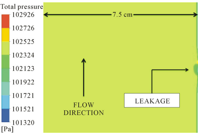
Figure 11. Pressure field near the leakage.
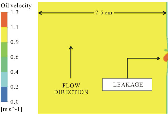
Figure 12. Oil velocity field near the leakage.
transported in the pipeline), since the time interval of pressure drop observed is very short (less than 0.03 s). This research revealed too that in heavy oil-water flow it is more easy to detect leaks when the pipe operate with high fluid velocities and greater water volume fraction in the mixture at the pipe inlet. It was verified that the oil volume fraction in the mixture affect strongly the spread and the exit direction of the oil in the leakage hole.
5. Acknowledgements
The authors would like to express their thanks to Brazilian researches agencies ANP/UFCG-PRH-25, CNPq, CAPES, FINEP and PETROBRAS S/A for supporting this work, and are also grateful to the authors of the references in this paper, that helped in the improvement of quality.
REFERENCES
- J. Y. Xu, D. H. Li, J. Guo and Y. X. Wu, “Investigations of Phase Inversion and Frictional Pressure Gradients in Upward and Downward Oil—Water Flow in Vertical Pipes,” International Journal of Multiphase Flow, Vol. 36, No. 11-12, 2010, pp. 930-939. doi:j.ijmultiphaseflow.2010.08.007
- S. I. Kam, “Mechanistic Modeling of Pipeline Leak Detection at Fixed Inlet Rate,” Journal of Petroleum Science and Engineering, Vol. 70, No. 3-4, 2010, pp. 145-156. doi:j.petrol.2009.09.008
- X. H. Lu, Y. J. Sang, J. Z. Zhang and Y. Y. Fan, “A Pipeline Leakage Detection Technology Based on Wavelet Transform Theory,” Proceedings of IEEE Annual International Conference on Information Acquisition, Shandong, 20-23 August 2006, pp. 1432-1437. doi:10.1109/ICIA.2006.305966
- R. Hu, H. Ye, G. Wang and C. Lu, “Leak Detection in Pipelines Based on PCA,” Proceedings of 8th International Conference on Control, Automation, Robotics and Vision, Kunming, 6-8 December 2004, pp. 1985-1989. doi:10.1109/ICARCV.2004.1469466
- H. V. Silva, C. K. Morooka, I. R. Guilherme, T. C. Fonseca and J. R. P. Mendes, “Leak Detection in Petroleum Pipelines Using a Fuzzy System,” Journal of Petroleum Science and Engineering, Vol. 49, No. 3-4, 2005, pp. 223-238. doi:j.petrol.2005.05.004
- L. Dong, S. Chai and B. Zhang, “Leak Detection and Localization of Gas Pipeline System Based on Wavelet Analysis,” Proceedings of 2nd IEEE International Conference on Intelligent, Control and Information Processing, Harbin, 25-28 July 2011, pp. 478-483. doi:10.1109/ICICIP.2011.6008290
- C. Verde, “Multi-Leak Detection and Isolation in Fluid Pipelines,” Control Engineering Practice, Vol. 9, No. 6, 2001, pp. 673-682. doi:10.1016/S0967-0661(01)00026-0
- C. G. Mothé and C. Silva, “Heavy-oil—Reserves and World Production,” TN Petróleo, Vol. 57, 2007, pp. 76-81. http://www.tnpetroleo.com.br/download.php/revista/download/i/33/nome/TN57_Artigos.pdf
- ANSYS, “CFX-Solver Theory Guide (Release 11.0),” ANSYS, Inc., Canonsburg, 2006.
NOTES
*Corresponding author.