Journal of Signal and Information Processing
Vol.07 No.03(2016), Article ID:68533,13 pages
10.4236/jsip.2016.73013
Comparison of Three Techniques to Identify and Count Individual Animals in Aerial Imagery
Pat A. Terletzky, Robert Douglas Ramsey
Department of Wildland Resources, Utah State University, Logan, USA

Copyright © 2016 by authors and Scientific Research Publishing Inc.
This work is licensed under the Creative Commons Attribution International License (CC BY).
http://creativecommons.org/licenses/by/4.0/


Received 9 May 2016; accepted 15 July 2016; published 18 July 2016
ABSTRACT
Whether a species is rare and requires protection or is overabundant and needs control, an accurate estimate of population size is essential for the development of conservation plans and management goals. Current wildlife surveys are logistically difficult, frequently biased, and time consuming. Therefore, there is a need to provide additional techniques to improve survey methods for censusing wildlife species. We examined three methods to enumerate animals in remotely sensed aerial imagery: manual photo interpretation, an unsupervised classification, and multi- image, multi-step technique. We compared the performance of the three techniques based on the probability of correctly detecting animals, the probability of under-counting animals (false positives), and the probability of over-counting animals (false negatives). Manual photo-interpretation had a high probability of detecting an animal (81% ± 24%), the lowest probability of over-count- ing an animal (8% ± 16%), and a relatively low probability of under-counting an animal (19% ± 24%). An unsupervised, ISODATA classification with subtraction of a background image had the highest probability of detecting an animal (82% ± 10%), a high probability of over-counting an animal (69% ± 27%) but a low probability of under-counting an animal (18% ± 18%). The multi- image, multi-step procedure incorporated more information, but had the lowest probability of detecting an animal (50% ± 26%), the highest probability of over-counting an animal (72% ± 26%), and the highest probability of under-counting an animal (50% ± 26%). Manual interpreters better discriminated between animal and non-animal features and had fewer over-counting errors (i.e., false positives) than either the unsupervised classification or the multi-image, multi-step techniques indicating that benefits of automation need to be weighed against potential losses in accuracy. Identification and counting of animals in remotely sensed imagery could provide wildlife managers with a tool to improve population estimates and aid in enumerating animals across large natural systems.
Keywords:
Aerial Photography, ISODATA, Principal Components, Texture, Unsupervised Classification

1. Introduction
Monitoring and detecting changes or trends in wildlife population abundance requires accurate enumeration of animals and has evolved from the simple counting of individuals in a given area [1] to the development of models estimating bias [2] , to complex, statistically based estimators and their associated correction factors [3] - [6] . Regardless of the type of survey conducted, counts in remote, hard to access locations or over extensive areas are logistically difficult to obtain, time consuming, and frequently biased [6] - [11] . Given the biases inherent to aerial and ground surveys and photographic interpretation, a method to identify and enumerate animals that is economical, repeatable, and accurate would provide wildlife managers another tool for estimating population abundances of wildlife species.
Counts of animals from remotely sensed imagery or aerial photographs have been used to estimate population abundances for a diverse array of wildlife species, from birds [12] - [15] to terrestrial species [16] [17] to oceanic mammals [18] [19] . Unfortunately, manual counts from aerial photographs are labor intensive, subject to human interpretation and error, and can result in inconsistent counts [12] [14] [20] - [22] . While manual counting of canvasbacks ducks (Aythya valisineria) on water in aerial photographs resulted in high variation among interpreters [12] , manual counting of caribou (Rangifer tarandus, [23] ) in open tundra habitatresulted in little variation in numbers of animals reported by independent interpreters. Although these studies found conflicting results, the types of errors indicate a link between body size and background conditions. A predominate trend across all studies enumerating animals in remotely sensed imagery was the importance of providing high contrast between animals and their background [10] [20] [24] - [28] . For example, snow geese (Chen caerulescens) are uniformly white-colored which facilitated separation of the birds from a darker background [20] . Snow provided a homogenous background and facilitated identification of deer (Odocoileus spp.) in remotely sensed images in the near infrared portion (NIR, 0.7 to 1.4 μm and 1.5 to 4.0 μm) of the electromagnetic spectrum (EM) but not in the visible region (0.5 to 0.7 μm [25] ). In the same study area in summer complex, non-homogenous backgrounds reduced the detection and identification of deer by 50% - 80% with higher detections achieved with less non-photosynthetic tissue (i.e., dry, brushy vegetation) surrounding the animal [24] . Large aggregations of birds have also been successfully counted in remotely sensed imagery, both as individual birds and as colonies. Greater flamingo (Phoenicopterus roseus) colonies were identified as overlapping ellipses that were unique in shape and spectrally distinct from the surrounding background [27] . The process was automated and resulted <5% difference when compared to manual counts. A supervised classification process with a combination of medium (10 m) and high resolution (61 cm and 2.44 m) imagery successfully identified and enumerated colonies of emperor penguins (Aptenodytes fosteri) across the continental coastline of Antarctica (approximately 18,000 km).
As the amount of available satellite and aerial imagery increases, there is a concomitant need for automated or semi-automated image analysis to reduce analysis time, allow non-photogrammetric specialists to interact with imagery, facilitate faster searches, and identify quantitative information not readily recognizable with human interpretation [29] - [31] . Similar to other research that identified and counted animals in remotely sensed imagery, our research was based on identifying and distinguishing features from the surrounding background. Our research is unique due to the integration of multiple data sources and the development of multi-dimensional analysis to increase the distinction between known animal pixels and known non-animal pixels. We developed a proof of concept using aerial imagery of fenced pastures containing known numbers of domestic cattle (Bos Taurus) and horses (Equus caballus). We examined one technique that relied solely on human interpretation (i.e., manual photo-interpretation) and two techniques that had minimal input from analysts: an ISODATA classification [32] with subtraction of a background image and a multiple image, multiple step technique. We compared the performance of the three techniques based on the probability of correctly detecting animals, the probability of under-counting animals (false negative), and the probability of over-counting animals (false positive). A correction factor integrating all detection probabilities adjusted the final count estimate for each image. The study was limited to grassland ecosystems due to the reduced complexity of cover as compared to dense, tall shrublands, and forests.
The advantages of counting animals from airborne or satellite imagery include reduced survey time, a permanent record of the survey, and potentially systematic errors which are more predictable when compared to conventional wildlife surveys. Conventional aerial wildlife surveys frequently require multiple days to complete thus allowing animals to move throughout the study area and increase the probability of double-counting or missing individuals. Remotely sensed imagery can be acquired over larger areas more quickly than conventional wildlife aerial surveys which are required to fly at slow speeds and at low elevations. In addition, flight restrictions may prevent aerial surveys over sensitive areas (i.e., military installations). The reduction in the amount of time needed to acquire remotely sensed imagery over that of a conventional wildlife survey could facilitate counting of animals in areas previously too large or too isolated to survey with traditional aerial survey methods. The permanent, unchanging record of animal locations for an instant in time (i.e. a complete count), allows for repeated assessments using new procedures developed with new technologies. Semi-automated counts of wildlife via remotely sensed imagery and the subsequent estimates of population size could revolutionize how ungulate counts are conducted and be a beneficial tool in management decisions. This method not only has the potential to improve accuracy and precision of counts and thus estimates of population size, it could aid in tracking grazing patterns of wild and domestic animals across large natural systems.
2. Study Areas
We acquired aerial imagery across portions of Cache County (i.e., Cache Valley) and a portion of Box Elder County in northcentral Utah. Cache Valley (CV) is a north-south trending valley surrounded by the Wellsville Mountains to the west and the Bear River Mountain Range to the east. Cache Valley has an average annual precipitation of 45 cm [33] with an elevation of 1355 m [34] in the center of the valley. Sites in CV were located in the valley bottomlands dominated by grasslands. Brigham City (BC) is located in Box Elder County and sits on the western base of the north-trending Wellsville Mountains. The average precipitation of the BC sites was 47 cm [33] with an elevation of 1289 m [34] . BC study sites were dominated by sparse grasslands.
3. Methodology
3.1. Aerial Imagery
On October 31, 2006, under mostly clear skies, we collected aerial imagery between 10:44 AM and 3:07 PM with three Kodak Megaplus 4.2i digital cameras (Kodak Company, Rochester, New York, New York) each recording a specific spectral region: green (0.54 - 0.56 µm), red (0.66 - 0.68 µm), and near-infrared (0.7 - 0.9 µm) with an approximate spatial resolution of 25 cm [35] . An Exotech four-band radiometer included with the cameras allowed for the conversion of digital numbers to reflectance values [36] . We acquired two images for each pasture, with at least 48 minutes between acquisitions of the first image (a) and the second image (b). Rectification of images to the Universal Transverse Mercator System (UTM), NAD83 datum occurred in ERDAS Imagine 9.1.0. (Leika Geosystems, Heerburg, Canton St. Gallen, Switzerland). Image acquisition likely did not affect animal movements since the aircraft flew at an average elevation of 549 m above ground level [37] [38] .
3.2. Animal Ground Counts
Rather than compare one estimate to another estimate, we compared the number of animals identified by each technique to the known number of animals in each pasture. Ground enumeration of cattle and horses occurred concurrently with image acquisition. Known counts of animals per pasture were derived from visual ground counts and available landowner counts (Figure 1). Pastures containing ≥50 animals were difficult to enumerate on the ground and resulted in unreliable counts, thus those pastures were not included in the analysis. Although no probability of detection was determined for the ground counts, by limiting analysis to those pastures with ≤50 animals, the detection probability was likely close to 100%. We considered pastures as independent samples since they were geographically separated across the study sites.
3.3. Accuracy Measures
The output from the manual photo-interpretation was an image containing circles around suspected animals (Figure 1). The two semi-automated techniques generated individual polygons for each suspected animal. We
 (a) (b)
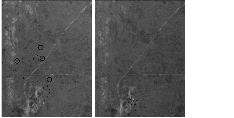
Figure 1. Images of the first (a) and second (b) acquisitions of pasture 15 indicating animal movement. Circles in (a) represent how a photo-interpreter would indicate which features were animals.
were able to evaluate when circled features (or polygons) were properly identified by comparing them against known animal locations. We classified polygons (or circles in the photo-interpretation) into three categories: “mapped polygons” consisted of all polygons generated in a particular technique, “correctly mapped” polygons were those generated using one of the three techniques that accurately depicted animals, and “incorrectly mapped” polygons were polygons not associated with a known animal. We assumed that features that moved location from one image to another image were animals and thus were able to determine a specific location for each animal. Because we knew specific locations of animals in each pasture, we were able to identify when an animal was not linked with a polygon (missed). Any animal not associated with a polygon was considered a “missed animal”.
The probability of detection (PD) is a proportion of correctly identified animals relative to a known number of animals [6] . In this paper, the PD calculation was defined as the number of correctly mapped polygons (or a circle in the photo-interpretation) divided by the number of known animals in the pasture. The probability of under-counting animals (Punder) indicated the proportion of animals known to be in a pasture but not associated with a polygon (or a circle in the photo-interpretation) identified and was calculated as the number of missed animals divided by the number of known animals in the pasture. The probability of over-counting (Pover) was calculated by dividing the number of polygons (or circles in the photo-interpretation) not associated with an animal by the number of mapped polygons (or circles in the photo-interpretation) in the pasture. We incorporated the three error estimates into a single correction factor (CF) that we multiplied by the number of mapped polygons to generate a population abundance estimate for each pasture. Abundance estimates, adjusted for false positives (over-counting animals) and false negatives (missed animals), have greater validity and are more robust than unadjusted estimates. The CF was calculated as (PD + Punder − Pover)/PD.
3.4. Interpretation Techniques
We evaluated the ability of five lay-people (L), five remote sensing analysts (R), and wildlife biologists (W) from the Utah Division of Wildlife Resources to count animals in aerial photographs of fenced pastures containing cattle. None of the individuals in the L group had any experience in remote sensing analysis or participated in wildlife surveys, none of the individuals in the R group participated in wildlife surveys, but some of the individuals in the W group had limited remote sensing experience (i.e., had previously examined remotely sensed imagery). All participants examined the same seven images of fenced pastures. The number of animals in each pasture ranged from five to 32. The photos of each pasture were presented to the photo-interpreters in natural color on a single standard 8.5 × 11-inch piece of paper. There was unlimited time for evaluation and individuals circled each feature interpreted as an animal (Figure 1). Although participants received pastures in the same order, the evaluation sequence was at the individual’s discretion. Due to the data being highly skewed across the three groups, the use of an ANOVA [39] was inappropriate. Log, squared, and square root transformations did not normalize these distributions. Additionally, a generalized linear model fit with a binomial distribution was not suitable since PD, Punder, and Pover were probabilities. Therefore, we used a Kruskal-Wallis test [39] to determine if there were significant differences in the probability of detection, the probability of under-counting, and the probability of over-counting animals. All statistical tests were conducted in the R statistical software [40] .
We used a semi-automated, multi-step technique to identify animals in remotely sensed imagery that included Iterative Self-Organizing Analysis Technique (ISODATA) segmentation (Figure 2(a)) and the generation of a background image (Figure 2(b)). Unsupervised classification, commonly used to segment and classify remotely sensed imagery, has the ability to identify unique features on the landscape and separates spectral information into distinct statistical clusters so that pixels with similar spectral characteristics are assigned to the same cluster [32] . One advantage of unsupervised classification is that it requires little analyst input beyond determination of the number of output clusters. The ISODATA process [32] [41] places a pixel into the cluster with the closest Euclidean spectral distance. The ISODATA segmentation generated 20 clusters from each 3-band image that were then converted into polygons, with each polygon assigned the mean spectral value of the pixels that it encompassed. We determined that clusters with the three lowest spectral values represented potential animal polygons (PAPs) and focused our subsequent analysis on these polygons (Figure 2(a)). We intersected the PAPs with the associated 3-band image to extract the original spectral response for each polygon to maintain as much spectral information as possible through the image differencing process.
Image differencing is a change detection technique in which an image collected at time X is subtracted from a second, geographically identical image, collected at time Y. In a differenced image, pixels with small spectral values represent areas that have changed little, while pixels with large spectral differences represent areas of change [32] . Generally, image differencing has been used to identify land-cover changes between images ac-
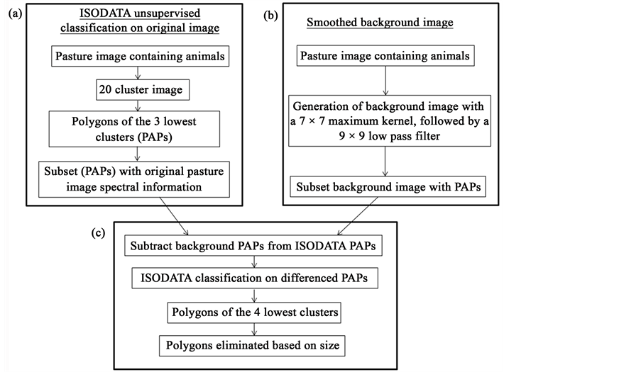
Figure 2. Outline of the steps taken in an ISODATA and background subtraction technique to identify animals in aerial imagery (a) Outlines generation of potential animal polygons (PAPs) from an unsupervised ISODATA process; (b) Outlines the background image generations; and (c) Outlines the subtraction of the ISODATA segmented image from the background image.
quired on two different dates [42] - [44] . Rather than the subtraction of temporally different images, we tested the feasibility of subtracting a simulated background image from an image containing animals to highlight differences between animal features and their surrounding background. As temporal image differencing detects changes over time, changes between a background image without animal features and an image of the same area with animal features should, in theory, isolate animal features. Since the ISODATA segmentation alone generated many false positives (i.e., over-counted animal features), we needed to further isolate animal features from the surrounding background. Based on a heuristic evaluation, we determined that low spectral values consistently represented animals. To generate a background image, we removed pixels with low spectral values (i.e., animal clusters) using a two-step process (Figure 2(b)). First, we applied a 7 × 7 maximum convolution kernel to the original image, which generated an image consisting of pixels with the highest spectral values in the kernel. Next, we applied a 9 × 9 low-pass filter to the maximum kernel image, which reduced spatial variation sufficiently to produce a smoothed background image. We then intersected the PAPs with the simulated background to generate pixel groupings that contained only background spectral values. We subtracted the PAP pixel groupings generated in the ISODATA step from the background pixel groups (Figure 2(c)). Based on image differencing theory, pixels in the subtracted image with higher difference values should represent animal polygons (i.e., animal spectral values subtracted from the background spectral values) and lower difference values should represent non-animal features (i.e., background spectral values subtracted from background spectral values. To further isolate animal features, a 20-class ISODATA segmentation was conducted on the differenced pixel groups. As with the previous 20-class ISODATA segmentation process, we heuristically identified pixels with the three lowest spectral values as representing animals. We eliminated pixel clusters with spectral values greater than the third lowest value and converted the remaining clusters to polygons. We heuristically identified spatial thresholds which described known animal shapes from the training images and removed polygons that were too large or too small to be animals.
Our third technique examined a multi-image, multi-step (MIMS) technique to isolate animals in remotely sensed imagery (Figure 3) with eight training images containing 143 animals and seven test images containing
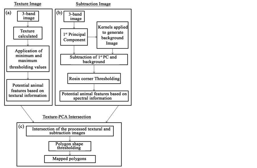
Figure 3. Outline of the steps taken in a multi-image, multi-step technique to identify animals in aerial imagery (a) Outlines generation of a texture image; (b) Outlines the principal components analysis (PCA) and background subtraction, and (c) Outlines the subtraction of the texture and PCA images.
158 animals. The training images were chosen so the number of animals in the training images was approximately the same as in the testing images. The MIMS technique generated three output images from each original 3-band pasture image: a texture image, the first principal component image, and a background image (see ISODATA methods above). Texture represents spatial change in spectral values within a specified neighborhood and therefore characterizes spatial patterns across an image [32] . Since texture quantifies variation within a neighborhood, we theorized that a neighborhood, which encompassed both an animal and its surrounding background, would exhibit greater variance (texture) than a neighborhood composed entirely of animal or background pixels. The size of a single bull can range from 1.6 to 2.2 m2 while the size of a single cow can range from 1.4 to 1.5 m2 (B. Bowman, personal communication); thus, an area of 1.5 m2 would encompass a small bull or a large cow. To generate a texture image, we used a neighborhood of 7 × 7 pixels (3.1 m2) that would theoretically encompass two animals standing next to each other. A mean Euclidean distance texture function representing the mean spectral difference between the central pixel and all other pixels in the neighborhood was used [41] . Neighborhoods with little spectral change resulted in low texture values while neighborhoods with many changes had higher texture values. To reduce heuristic determination of thresholding values and thus increase potential for automation, we defined the minimum texture thresholding value based on the Rosin corner threshold technique (Figure 4) [45] . We removed non-animal pixels that were above the maximum texture threshold and below the minimum texture threshold and converted pixel clusters into polygons. Principal components analysis (PCA) is commonly used with remotely sensed imagery to reduce dimensionality by combining redundant information in highly correlated bands [32] [46] . The output of a PCA is an image, which is composed of the same number of layers as the input image (3 bands in this case). The first PCA layer contains the highest amount of correlated information between the spectral bands and the second layer contains the second highest amount of correlated information and so on [32] . We conducted a PCA on each 3-band training image and used the first principal component for subsequent analysis because it contained the highest amount of spectral variation (81% vs. 17% and 2%, 1st, 2nd, and 3rd components, respectfully). We subtracted the background image derived from our ISODATA methods (Figure 2(b)) from the first principal component (Figure 3(b)) and applied the Rosin corner thresholding method to eliminate non-animal features. We spatially intersected the texture

Figure 4. Graphical depiction of the Rosin corner method of determining a thresholding values for a histogram of texture values from an image containing animals. The peak of the histogram is the starting point of a straight lines that ends at the first instance of an X-axis value of zero. The dashed line perpendicular to the straight line with the longest distance to the histogram curve is the threshold value.
derived polygons (Figure 3(a)) with polygons derived from the PCA-background subtraction technique (Figure 3(b)) and considered the spatial locations where both polygons intersected as an animal. The final step eliminated polygons based on thresholding values for area, perimeter-area ratio (PA), and compactness ratio (CR; Figure 3(c)). We examined the PA to assess the circularity of a feature relative to a perfect circle. The CR also assesses the circularity of a feature but without influence of feature size, unlike PA. We heuristically determined thresholds of shape characteristics that encompassed animal features from the training imagers. Individual shape characteristics alone were unable to successfully threshold animal features so we used a combination of all three characteristics to eliminate non-animal polygons. The final output resulted in polygons classified as animal features.
4. Results and Discussion
There were no significant differences (p ≥ 0.20) among individuals that manually interpreted the aerial imagery within the L, W, or R groups for PD, Punder, or Pover, so we collapsed individuals within each group and examined differences among the groups. There were no significant differences among the three groups for PD, Punder, and Pover (p ≥ 0.10, Figure 5). Collapsing across groups, the overall mean PD was 83% (±1%, Standard error), the mean Punder was 19% (±1%), the mean Pover was 8% (±3%), and the mean CF was 1.26 (±0.07).
The mean PD for the seven pastures examined with the ISODATA and background image subtraction was 82% (±10%, SD) and ranged from 55% to 100% (Table 1). The mean Punder for the seven pastures was 18% (±18%) and ranged from 0% to 45%. The mean Pover for the seven images was 69% (±27%) and ranged from 28% to 98%. The mean CF for the seven images was 0.40 (±0.37) and ranged from 0.04 to 0.91. The ISODATA unsupervised classification with a background subtraction successfully identified animals but greatly over-estimated

Figure 5. Graphs indicating no significant difference (p ≥ 0.05) among laymen (L), remote sensing analysts (R), and wildlife biologists (W) for the probability of detecting an animal, the probability of under-counting animals, the probability of over- counting animals, and a correction factor in aerial imagery of fenced pastures containing animals.
animal numbers. While there appeared to be a positive relationship between increasing number of known animals in a pasture with increasing number of animals missed and increasing CF’s, there was no significant relationship (p > 0.05) between the actual number of animals in each pasture and any image feature characteristic (i.e., total number of polygons in an image, PD, Punder, Pover, or CF).
The MIMS technique was similar to the ISODATA-background subtraction technique in that there was a general trend without significance (p > 0.05) for the number of missed animals to increase as the number of known animals in a pasture increased. The mean PD across the testing pastures was 50% (±26%) and ranged from 0% to 74%. The mean Punder for the testing pastures was 50% (±26%) and ranged from 26% to 100%. The mean Pover was 72% (±26%) and ranged from 23% to 100%. The mean CF was 0.54 (±32) and ranged from 0.24 to 1.09 (Table 2).
The PD is generally calculated as the ratio of the number of marked animals observed during a wildlife survey to the known number of marked animals on the survey area. Reported values of PD for conventional ground and

Table 1. The probabity of detecting an animal (PD), the probability of under-counting an animal (Punder), the probability of over-counting an animal (Punder), and the correction factor (CF) for an ISODATA and background subtraction techinque to identify animals in aerial imagery in fenced pastures in northcentral Utah.
a(Correctly mapped polygons/Known number of animals in pasture); b(Missed Animals / Known number of animals in pasture); c(Incorrectly mapped polygons/Number of mapped polygons); d(PD + Punder − Pover)/PD.
Table 2. The probabity of detecting an animal (PD), the probability of under-counting an animal (Punder), the probability of over-counting an animal (Punder), and the correction factor (CF) for a multi-imge, multi-step (MIMS) technique to identfy and count animals in remotely sensed imagery across seven pastures in northcentral Utah.
a(Correctly mapped polygons / Known number of animals in pasture); b(Missed Animals/Known number of animals in pasture); c(Incorrectly mapped polygons/ Number of mapped polygons); d(PD + Punder − Pover)/PD; eOne polygon represented 2 animals.
aerial surveys range from 52% in caribou (Rangifer spp., [47] ), 34% - 82% for mule deer (Odocoileus hemionus, [48] ), and 53% - 71% for feral ungulate species [49] ). The mean PD of 50% for the MIMS procedure is within reported levels of the PD for wildlife surveys but indicates that the technique would detect only 50% of the animals present in an image. The mean PD of the manual interpretation and the ISODATA procedures, 81% and 82%, respectively, are above reported levels for ground and aerial surveys. The higher variability of the PD of the manual interpretation compared to the semi-automated, ISODATA technique (Table 3) is similar to reported photo-interpretation values [12] [21] ) and supports the contention that manual counts are inconsistent and thus estimates derived from them should consider those inconsistencies. The coefficient of variation (CV) is a measure of variation that is normalized with respect to the mean of a data set [39] and is an appropriate statistic to compare the amount of variation from one technique to another especially when there is a wide range in the mean values examined. The CV for the probability of detection for the ISDODATA technique is 12%, 30% for the manual photo-interpretation, and 52% for the MIMS technique indicating that the ISODATA has the lowest variance relative to the mean, followed by manual photo-interpretation, and the MIMS had the highest variance.
Manual interpreters were better able to discriminate between animal and non-animal features and identified fewer over-counting errors (i.e., false positives) than either the ISODATA or the MIMS techniques (Table 3). Most individuals had a CF of 1.00 for at least a single image indicating no correction to the number of animals enumerated was needed. The interpreters were better able to distinguish between animal and non-animal features likely due to their ability to integrate qualitative information concerning spectral information and shape characteristics [50] . Human vision evaluates features in a qualitative and comparative manner and integrates multiple dimensions of information to discern features [30] [50] . The multi-step techniques incorporated into both the ISODATA and MIMS procedures attempted to isolate and refine new information at each step. For example, the texture image generated in the MIMS technique (Figure 2) was an attempt to isolate and categorize the differences within a neighborhood similar to how human vision might qualify spectral differences in an area of interest. The fact that the MIMS had the lowest PD coupled with the highest Punder and Pover suggests that increased complexity does not equate to increased accuracy nor does it represent how humans evaluate imagery.
The MIMS technique identified too few polygons as animals in 3 pastures which resulted in a low PD (Table 2) due to polygons that were correctly associated with animal features initially but at later steps were erroneously eliminated. The MIMS removed polygons at three steps: 1) via the Rosin corner thresholding method on spectral values (Figure 4), 2) due to thresholding of the texture image, and 3) due to thresholding of shape and size characteristics. Incorrect removal of polygons at each stage was not consistent across all pastures. The Rosin thresholding method incorrectly removed polygons that represented animals in a single pasture but not in other pastures. The shape thresholding incorrectly removed polygons from 2 pastures because they were outside the shape thresholding values. Some animal features (i.e., polygons) included shadow pixels which increased the area of the polygon beyond the size threshold.
5. Conclusions
Our objective was to compare how manual interpretation, an ISODATA unsupervised classification with background subtraction process, and a multi-image, multi-step technique were able to identify and count individual animals in aerial imagery. Manual interpretation of remotely sensed imagery, regardless of prior knowledge or experience of the interpreters, resulted in higher detection probabilities, and lower under- or over-counting of animal when compared to an ISODATA unsupervised classification or a multi-image, multi-step process. All
Table 3. The mean and standard deviation of the probability of detecting an animal (PD), the probability of under-counting an animal (Punder), the probability of over-counting an animal (Punder), and the correction factor (CF) for the count estimate of three techniques to identify animals in remotely sensed imagery from northcentral Utah.
a(Correctly mapped polygons/Known number of animals in pasture); b(Missed Animals/Known number of animals in pasture); c(Incorrectly mapped polygons/Number of mapped polygons); d(PD + Punder − Pover)/PD.
interpreters were able to discriminate between non-animal and animal features by integrating qualitative information derived from spectral and shape characteristics in a comparative process. In an attempt to emulate the human ability to integrate multiple dimensions of contextual information, we explored techniques that integrated spatial and spectral information to isolate animal features in remotely sensed imagery. Employing conventional remote sensing techniques, an ISODATA unsupervised classified image subtracted from a simulated background image was used to highlight differences in areas containing animals compared to differences in areas without animals. The ISODATA technique had a similar detection probability as manual interpretation but greatly over estimated the number of animals, resulting in counts that required the most correction of all 3 techniques. If animals were present in an image, the ISODATA technique correctly identified most of the animals but greatly over-estimated numbers. Additional information was needed to reduce over-counting errors while maintaining low under-counting errors. A multi-dimensional technique attempted to reduce over-counting errors by integrating texture images, principal components analysis, heuristic thresholding, and image subtraction. The first principal component provided the highest amount of spectral information (i.e., the most variation) and was the basis for the MIMS technique. Contrary to the ISODATA technique, the MIMS errors of under-counting were high but like the ISODATA technique, errors of over-counting also were high. Consideration of the PD alone indicated the manual interpretation and ISODATA techniques would identify animals if they were present in an image, with the ISODATA technique being more consistent. The high Pover for the ISODATA and MIMS techniques indicate the enumeration would be overestimated with semi-automated techniques but less so with the manual photo-interpretation. Thus, the ISODATA technique will identify 80% of the animals in remotely sensed imagery, but it will overestimate the number of animals present due to consistent over-counting.
The advantages of airborne or satellite imagery to count animals include reduced survey time, a permanent record of the survey, and potentially cost less than conventional wildlife surveys. The reduction in time required to acquire remotely sensed imagery of a large study area could facilitate counting of animals in areas previously too large or too isolated to survey. The permanent, unchanging record of animal locations for an instant in time allows for repeated assessments using new techniques or even new technologies. Identification and counting wildlife in remotely sensed imagery could revolutionize how wildlife surveys are conducted and be a beneficial tool in management of wildlife populations by providing improved estimates of population size. This method not only has the potential to improve accuracy and precision of counts and thus estimates of population size, it could aid in tracking grazing patterns of wild and domestic animals across large natural systems.
Acknowledgements
We thank the lay people, remote sensing analysts, and wildlife biologists for volunteering their time to participate in the manual photographic interpretation. This research was supported by the Utah Agricultural Experiment Station, Utah State University, and approved as journal paper number 8910.
Cite this paper
Pat A. Terletzky,Robert Douglas Ramsey, (2016) Comparison of Three Techniques to Identify and Count Individual Animals in Aerial Imagery. Journal of Signal and Information Processing,07,123-135. doi: 10.4236/jsip.2016.73013
References
- 1. Leopold, A., Sowls, L.K. and Spencer, D.L. (1947) A Survey of Over-Populated Deer Ranges in the United States. Journal of Wildlife Management, 11, 162-177.
http://dx.doi.org/10.2307/3795561 - 2. Caughley, G. (1974) Bias in Aerial Survey. Journal of Wildlife Management, 38, 921-933.
http://dx.doi.org/10.2307/3800067 - 3. Garton, E.O., Ratti, J.T. and Giudice, J.H. (2005) Research and Experimental Design. In: Braun, C.E., Ed., Techniques for Wildlife Investigations and Management, The Wildlife Society, Bethesda, 43-71.
- 4. Gregory, R.D., Gibbons, D.W. and Donald, P.F. (2004) Bird Census and Survey Techniques, Bird Ecology and Conservation: A Handbook of Techniques. Oxford University Press, Oxford.
- 5. McComb, B., Zuckerberg, B. Vesely, D. and Jordan, C. (2010) Monitoring Animal Populations and Their Habitats: A Practitioner’s Guide. CRC Press, Boca Raton.
http://dx.doi.org/10.1201/9781420070583 - 6. Williams, B.K., Nichols, J.D. and Conroy, M.J. (2002) Analysis and Management of Animal Populations. Academic Press, San Diego.
- 7. Bartmann, R.M., White, G.C., Carpenter, L.H. and Garrott, R.A. (1987) Aerial Mark-Recapture Estimates of Confined Mule Deer in Pinyon-Juniper Woodland. Journal of Wildlife Management, 51, 41-46.
http://dx.doi.org/10.2307/3801626 - 8. Brockett, B.H. (2002) Accuracy, Bias and Precision of Helicopter-Based Counts of Black Rhinoceros in Pilanesberg National Park, South Africa. South African Journal of Wildlife Research, 32, 121-136.
- 9. Jackmann, H. (2002) Comparison of Aerial Counts with Ground Counts for Large African Herbivores. Journal of Applied Ecology, 39, 841-852.
http://dx.doi.org/10.1046/j.1365-2664.2002.00752.x - 10. Storm, D.J., Samuel, M.D., Van Deelen, T.R., Malcolm, K.D., Rolley, R.E., Frost, N.A., et al. (2011) Comparison of Visual-Based Helicopter and Fixed-Wing Forward-Looking Infrared Surveys for Counting White-Tailed Deer Odocoileus virginianus. Wildlife Biology, 17, 431-440.
http://dx.doi.org/10.2981/10-062 - 11. White, G.C., Bartmann, R.M., Carpenter, L.H. and Garrott, R.A. (1989) Evaluation of Aerial Line Transects for Estimating Mule Deer Densities. Journal of Wildlife Management, 53, 625-635.
http://dx.doi.org/10.2307/3809187 - 12. Erwin, R.M. (1982) Observer Variability in Estimating Numbers: An Experiment. Journal of Field Ornithology, 53, 159-167.
http://www.jstor.org/stable/4512706 - 13. Fretwell, P.T., LaRue, M.A., Morin, P., Kooyman, G.L., Wienecke, B., Ratcliffe, N., et al. (2012) An Emperor Penguin Population Estimate: The First Global, Synoptic Survey of a Species from Space. PLoS ONE, 7, e33751.
http://dx.doi.org/10.1371/journal.pone.0033751 - 14. Gilmer, D.S., Brass, J.A., Strong, L.L. and Card, D.H. (1988) Goose Counts from Aerial Photographs Using an Optical Digitizer. Wildlife Society Bulletin, 16, 204-206.
http://www.jstor.org/stable/3782190 - 15. Harris, M.P. and Lloyd, C.S. (1977) Variation in Counts of Seabirds from Photographs. British Birds, 70, 200-205.
- 16. Lubow, B.C. and Ransom, J.I. (2009) Validating Aerial Photographic Mark-Recapture for Naturally Marked Feral Horses. Journal of Wildlife Management, 73, 1420-1429.
http://dx.doi.org/10.2193/2008-538 - 17. Russell, J., Couturier, S., Sopuck, L.G. and Ovaska, K. (1996) Post-Calving Photo-Census of the Rivière George Caribou Herd in July 1993. Rangifer, 9, 319-330.
http://dx.doi.org/10.7557/2.16.4.1273 - 18. Hiby, A.R., Thompson, D. and Ward, A.J. (1988) Census of Grey Seals by Aerial Photography. The Photogrammetric Record, 12, 589-594.
http://dx.doi.org/10.1111/j.1477-9730.1988.tb00607.x - 19. Koski, W.R., Zeh, J., Mocklin, J., Davis, A.R., Rugh, D.J., George J.C., et al. (2010) Abundance of Bering-Chukchi- Beaufort Bowhead Whales (Balaena mysticetus) in 2004 Estimated from Photo-Identification Data. Journal of Cetacean Research and Management, 11, 89-99.
- 20. Bajzak, D. and Piatt, J.F. (1990) Computer-Aided Procedure for Counting Waterfowl on Aerial Photographs. Wildlife Society Bulletin, 18, 125-129.
http://www.jstor.org/stable/3782125 - 21. Frederick, P.C., Hylton, B., Heath, J.A. and Ruane, M. (2003) Accuracy and Variation in Estimates of Large Numbers of Birds in Individual Observers Using an Aerial Survey Simulator. Journal of Field Ornithology, 74, 281-287.
http://dx.doi.org/10.1648/0273-8570-74.3.281 - 22. Sinclair, A.R.E. (1973) Population Increases of Buffalo and Wildebeest in the Serengeti. East African Wildlife Journal, 11, 93-107.
http://dx.doi.org/10.1111/j.1365-2028.1973.tb00075.x - 23. Couturier, S., Courtois, R., Crépeau, H., Rivest, L.-P. and Luttich, S. (1994) Calving Photocensus of the Rivière George Caribou Herd and Comparison with an Independent Census. Proceedings of the 6th North American Caribou Workshop, Prince George, 1-4 March 1994, 283-296.
- 24. Trivedi, M.M., Wyatt, C.L. and Anderson, D.R. (1982) A Multispectral Approach to Remote Detection of Deer. Photogrammetric Engineering and Remote Sensing, 48, 1879-1889.
- 25. Wyatt, C.L., Trivedi, M.M., Anderson, D.R. and Pate, M.C. (1985) Measurement Techniques for Spectral Characterization for Remote Sensing. Photogrammetric Engineering and Remote Sensing, 51, 245-251.
- 26. Potvin, F., Breton, L. and Rivest, L. (2004) Aerial Surveys for White-Tailed Deer with the Double-Count Technique in Québec: Two 5-Year Plans Completed. Wildlife Society Bulletin, 32, 1099-1107.
http://www.jstor.org/stable/3784747
http://dx.doi.org/10.2193/0091-7648(2004)032[1099:asfwdw]2.0.co;2 - 27. Descamps, S., Béchet, A., Descombes, X., Arnaud, A. and Zerubia, J. (2011) An Automatic Counter for Aerial Images of Aggregations of Large Birds. Bird Study, 58, 302-308.
http://dx.doi.org/10.1080/00063657.2011.588195 - 28. Laliberte, A.S. and Ripple, W.J. (2003) Automated Wildlife Counts from Remotely Sensed Imagery. Wildlife Society Bulletin, 31, 362-371.
http://www.jstor.org/stable/3784314 - 29. Aitkenhead, M.J. and Aalders, I.H. (2011) Automating Land Cover Mapping of Scotland Using Expert System and Knowledge Integration Methods. Remote Sensing of Environment, 115, 1285-1295.
http://dx.doi.org/10.1016/j.rse.2011.01.012 - 30. Baraldi, A. and Boschetti, L. (2012) Operational Automatic Remote Sensing Image Understanding Systems: Beyond Geographic Object-Based and Object-Oriented Image Analysis (GEOBIA/GEOOIA). Part 1: Introduction. Remote Sensing, 4, 2694-2735.
http://dx.doi.org/10.3390/rs4092694 - 31. Walter, V. and Luo F. (2012) Automatic Interpretation of Digital Maps. Journal of Photogrammetry and Remote Sensing, 66, 519-528.
http://dx.doi.org/10.1016/j.isprsjprs.2011.02.010 - 32. Jensen, J.R. (2005) Introductory Digital Image Processing: A Remote Sensing Perspective. 3rd Edition, Prentice Hall, Upper Saddle River.
- 33. Moller, A.L. and Gillies, R.R. (2008) Utah Climate. 2nd Edition, Utah Climate Center, Utah State University Research Foundation, Logan.
- 34. US Geological Survey (1981) Geographic Names Information System (GNIS).
http://geonames.usgs.gov/pls/gnispublic - 35. Cai, B. and Neale, C.M.U. (1999) A Method for Constructing 3-Dimensional Models from Airborne Imagery. Proceedings of the 17th Biennial Workshop: Color Photography and Videography for Resource Assessment, Bethesda, 5-7 May 1999.
- 36. Neale, C.M.U. and Crowther, B.G. (1994) An Airborne Multispectral Video/Radiometer Remote Sensing System: Development and Calibration. Remote Sensing of Environment, 49, 187-194.
http://dx.doi.org/10.1016/0034-4257(94)90014-0 - 37. Bernatas, S. and Nelson, L. (2004) Sightability Model for California Bighorn Sheep in Canyonlands Using Forward- Looking Infrared (FLIR). Wildife Society Bulletin, 32, 638-647.
http://www.jstor.org/stable/3784786 - 38. De Young, C.A. (1985) Accuracy of Helicopter Surveys of Deer in South Texas. Wildlife Society Bulletin, 13, 146-149.
http://www.jstor.org/stable/3781428 - 39. Zar, J.H. (1996) Biostatistical Analysis. 3rd Edition, Simon & Schuster, Upper Saddle River.
- 40. R Core Development Team (2012) R: A Language and Environment for Statistical Computing. R Foundation for Statistical Computing, Vienna, Austria.
- 41. ERDAS (2003) ERDAS Field Guide. 7th Edition, Leica GeoSystems, Atlanta.
- 42. Key, T., Warner, T.A., McGraw, J.B. and Fajvan, M.A. (2001) A Comparison of Multispectral and Multitemporal Information in High Spatial Resolution Imagery for a Classification of Individual Tree Species in a Temperate Hardwood Forest. Remote Sensing of Environment, 75, 100-112.
http://dx.doi.org/10.1016/S0034-4257(00)00159-0 - 43. Lu, D., Mausel, P., Batistella, M. and Moran, E. (2005) Land-Cover Binary Change Detection Methods for Use in the Moist Tropical Region of the Amazon: A Comparative Study. International Journal of Remote Sensing, 26, 101-114.
http://dx.doi.org/10.1080/01431160410001720748 - 44. Lu, D., Mausel, P., Batistella, M. and Moran, E. (2004) Change Detection Techniques. International Journal of Remote Sensing, 25, 2365-2407.
http://dx.doi.org/10.1080/0143116031000139863 - 45. Rosin, P.L. (2001) Unimodal Thresholding. Pattern Recognition, 34, 2083-2096.
http://dx.doi.org/10.1016/S0031-3203(00)00136-9 - 46. Chavez Jr., P.S. and Kwarteng, A.Y. (1989) Extracting Spectral Contrast in Landsat Thematic Mapper Image Data Using Selection Principal Components Analysis. Photogrammetric Engineering & Remote Sensing, 55, 339-348.
- 47. Rivest, L., Couturier, S. and Crepeau, H. (1998) Statistical Methods for Estimating Caribou Abundance Using Post Calving Aggregations Detected by Radio Telemetry. Biometrics, 54, 865-876.
http://dx.doi.org/10.2307/2533841 - 48. Freddy, D.J., White, G.C., Kneeland, M.C., Kahn, R.H., Unsworth, J.W., et al. (2004) How Many Mule Deer Are There? Challenges of Credibility in Colorado. Wildlife Society Bulletin, 32, 916-927.
http://www.jstor.org/stable/3784816
http://dx.doi.org/10.2193/0091-7648(2004)032[0916:HMMDAT]2.0.CO;2 - 49. Bayliss, P. and Yeomans, K.M. (1989) Correcting Bias in Aerial Survey Population Estimates of Feral Livestock in Northern Australia Using the Double-Count Technique. The Journal of Applied Ecology, 26, 925-933.
http://dx.doi.org/10.2307/2403702 - 50. Russ, J.C. (1999) The Image Processing Handbook. 3rd Edition, CRC Press, Boca Raton.