Journal of Signal and Information Processing
Vol.5 No.2(2014), Article ID:45989,10 pages DOI:10.4236/jsip.2014.52006
Noise Removal in Speech Processing Using Spectral Subtraction
Marc Karam1, Hasan F. Khazaal2, Heshmat Aglan3, Cliston Cole1
1Department of Electrical Engineering, Tuskegee University, Tuskegee, USA
2Department of Electrical Engineering, Wasit University, Wasit, Iraq
3Department of Mechanical Engineering, Tuskegee University, Tuskegee, USA
Email: karam@mytu.tuskegee.edu
Copyright © 2014 by authors and Scientific Research Publishing Inc.
This work is licensed under the Creative Commons Attribution International License (CC BY).
http://creativecommons.org/licenses/by/4.0/


Received 14 January 2014; revised 14 February 2014; accepted 28 February 2014
ABSTRACT
Spectral subtraction is used in this research as a method to remove noise from noisy speech signals in the frequency domain. This method consists of computing the spectrum of the noisy speech using the Fast Fourier Transform (FFT) and subtracting the average magnitude of the noise spectrum from the noisy speech spectrum. We applied spectral subtraction to the speech signal “Real graph”. A digital audio recorder system embedded in a personal computer was used to sample the speech signal “Real graph” to which we digitally added vacuum cleaner noise. The noise removal algorithm was implemented using Matlab software by storing the noisy speech data into Hanning time-widowed half-overlapped data buffers, computing the corresponding spectrums using the FFT, removing the noise from the noisy speech, and reconstructing the speech back into the time domain using the inverse Fast Fourier Transform (IFFT). The performance of the algorithm was evaluated by calculating the Speech to Noise Ratio (SNR). Frame averaging was introduced as an optional technique that could improve the SNR. Seventeen different configurations with various lengths of the Hanning time windows, various degrees of data buffers overlapping, and various numbers of frames to be averaged were investigated in view of improving the SNR. Results showed that using one-fourth overlapped data buffers with 128 points Hanning windows and no frames averaging leads to the best performance in removing noise from the noisy speech.
Keywords:Speech Processing, Spectral Subtraction, Noise Removal, Fast Fourier Transform, Inverse Fast Fourier Transform

1. Introduction
Speech communications are used daily in our lives. Every case of speech communication involves a speaker, a listener, and various communication devices. Speech communications take place everywhere, such as domestic homes, work, school conferences, seminars, medical appointments, and cocktail parties. Often, random noises corrupt the communication between the speaker and the listener. These noises can cause speech to be heard incorrectly. Noises exist everywhere, and are produced by many factors, so that it is impossible to identify them all. The characteristics of these noises are either known or unknown; however, they all can distort, disrupt, or disguise the quality of speech signals. Therefore, background noises and noisy environments are likely to affect many people, especially people with hearing loss. The area of research that investigates removing noise from corrupted speech utilizing various signal processing methods is called speech processing. There are many different forms of speech processing such as speech enhancement, speech recognition, speech coding, and speech synthesis.
In recent studies, numerous filter designs have been implemented in communication systems to reduce and eventually eliminate the effects of incoming background noise, as well as to enhance speech intelligibility [1] -[5] . Removal of high frequency noise for speech enhancement using Frequency Response Masking (FRM), a technique based on designing low complexity, narrow transition bandwidth, linear phase Finite Impulse Response (FIR) filters, has been implemented [1] . An FIR filter has been designed to have impulse responses associated with various cut-off frequencies leading to a decrease in the Mean Square Error (MSE) when comparing original and filtered speech signals [2] . In applications where both the speech and the noise signals change continuously, adaptive filtering based on using three algorithms: Least Mean Square (LMS), Normalized Least Mean Square (NLMS), and Sign-Data Least Mean Square (SDLMS) algorithms has been implemented [3] . Discrete Wavelet Transform (DWT) algorithm was used for speech signal denoising with both hard and soft thresholding, with soft thresholding performing better than hard thresholding at all input SNR levels [4] . Residual musical noise resulting from spectral subtraction technique has been reduced using scaling factors and weighted functions [5] .
In this research, we focused on spectral subtraction noise removal approach in speech processing [6] . Our experiment involved sampling two different signals: a real-time speech signal “Real graph” and a noise signal generated by a vacuum cleaner. Using Matlab, we digitally added the vacuum cleaner noise to the speech signal “Real graph”, thus obtaining a noisy speech signal. Noise removal cannot be successfully implemented in the time domain; rather, it is performed in the frequency domain. Our spectral subtraction noise removal approach involves segmenting the noisy speech signal into half-overlapped time domain data buffers multiplied by a Hanning window and then transforming the result into the frequency domain using the fast Fourier transform (FFT). Subsequently, noise is removed by subtracting the average magnitude of the noise spectrum from the noisy speech spectrum and zeroing out the negative values using half-wave rectification. Finally, after removing the noise from the noisy speech, we reconstructed the noise-reduced speech back to time domain using the Inverse Fast Fourier Transform (IFFT) [7] . We were able to listen to the reconstructed speech and we observed that the noise had effectively been reduced. Statistical evaluation of the results was accomplished by calculating the Speech to Noise Ratio (SNR) [8] . In order to improve the performance, we applied the technique of frames averaging [9] . Moreover, we studied the effect of varying the overlapping lengths of the data buffers and the Hanning windows on improving the SNR.
2. Time Domain to Frequency Domain Conversion Using FFT
2.1. Sampling of the Noisy Speech “Real Graph” by Using the A-to-D Converter
First, consider the clean speech “Real graph” S(t) corrupted by vacuum cleaner noise N(t) and shown in Figure 1. The noisy speech “Real graph” is a continuous-time function which is converted to an electrical signal X(t) using a microphone connected to a digital audio recorder system. The microphone performs this conversion by detecting the changing air pressure of the audio sound. The electrical signals are transmitted through a cable wire or a median that is connected between the microphone and the digital audio recorder system.
The digital audio recorder system is an example of an Analog-to-Digital (A-to-D) converter. The A-to-D converter transforms the continuous-time noisy speech into a discrete-time noisy speech X[n]. A discrete-time signal is a non-continuous time signal. It has been sampled from a continuous-time signal using a digital audio recorder system. Discrete-time signals symbolize an indexed sequence of discrete-time samples. A continuoustime signal is sampled at equally spaced time impulses tn = nTs as follows
 , (1)
, (1)
where Ts is the sampling period or fixed time between each sample. Each impulse value of X[n] is called sample of the discrete-time signal. The sampling period can also be represented as a fixed sampling rate:
 . (2)
. (2)
In this research, a clean speech “Real graph” S[n] was recorded using software called sound recorder that was installed on a personal computer. A time waveform of the speech “Real graph” is shown in Figure 2(a).
The speech was recorded for a duration of 645 ms. Shannon sampling theorem states that any continuous-time signal with maximum spectrum frequency fmax can be reconstructed exactly from its samples X[n] = X(nTs) if the samples are taken at a sampling rate that is greater than 2 fmax. Since audio frequencies of audible sounds range from 20 to 20,000 Hz, thus, in our application, fmax is approximately 20 kHz. The sampling rate was automatically computed by Matlab, and had the value 44.1 kHz, which is bigger than twice 20 kHz, and thus satisfies the Shannon sampling theorem. There are a total of 28,446 samples with time space interval of 22.67 μs between each sample. A time waveform of a vacuum cleaner noise N[n] was also sampled for 645 ms at a rate of 44.1 kHz and is shown in Figure 2(b). The vacuum cleaner noise was digitally added to the clean speech. The sum of the two signals generates the noisy speech signal “Real graph” X[n] shown in Figure 2(c).
2.2. Storing the Noisy Speech “Real Graph” Using the Half-Overlapped Data Buffers
The noisy speech is the data we want to evaluate for noise removal. Once Matlab retrieves, reads, and formats
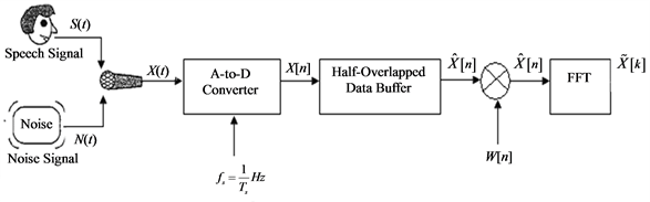
Figure 1. Block diagram of noisy speech generation and discretization.
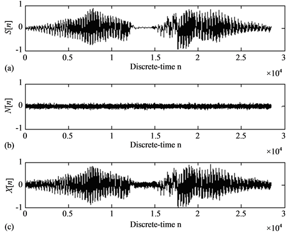
Figure 2. (a) Clean speech “Real graph” signal S(n); (b) Vacuum cleaner noise signal N(n); (c) Noisy speech “Real graph” corrupted by the vacuum cleaner noise X(n).
the data in numerical value, the data are stored into segments. Each segment contains 256 samples of the noisy speech. Each segment is called a data-buffer . Each data buffer half-overlaps another data buffer by a total of 128 samples. Our noisy speech “Real graph” has 221 half-overlapped data buffers that cover the entire length of the noisy speech data.
2.3. Analyzing the Noisy Speech “Real Graph” Using the Hanning Time Window
The noisy speech data of the 221 half-overlapped data buffers contain 28,446 samples; the transformation of the 28,446 samples from time domain to frequency domain using FFT would take a very long time for the computer to process and compute the spectrum. Computing a smaller amount of data at a time optimizes the efficiency of the computer processing speed. In this research, the noisy speech data of the 221 half-overlapped data buffers were decomposed into time windows called Hanning time windows. The Hanning time window is a bell curve shape that multiplies the noisy speech data of the half-overlapped data buffers. The portions of the noisy speech data that lie outside the Hanning time window are zeroed-out, while the portions inside are further evaluated for processing. The mathematical general expression of a Hanning time window is in the form
 , (3)
, (3)
where L is the length or the number of samples of the Hanning time window. The data that are stored in the Hanning time window are evaluated for spectral computation, which involves computing the discrete Fourier transform (DFT) using the FFT algorithm, as described in the next section.
3. Noise Removal in Frequency Domain and Conversion to the Time Domain Using IFFT
In this section, we present our algorithm for the spectral subtraction of noise from a speech signal [6] . A flowchart of this algorithm is shown in Figure 3. In the subsection below, we explain the role of the various blocks of this flowchart.
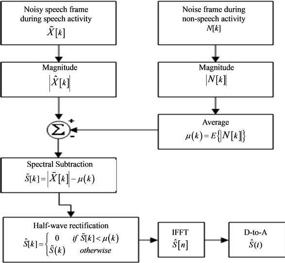
Figure 3. Spectral subtraction noise removal flowchart.
3.1. Speech and Non-Speech Activity Frame
Previously we discussed how we recorded two signals, a clean speech S[n] and a vacuum cleaner noise N[n]. The vacuum cleaner noise was digitally added to the clean speech to form a noisy speech X[n]. Appending X[n] to N[n], we composed the signal NX[n] shown in Figure 4(a). The first part of the signal is composed of the non-speech activity that contains the stationary noise of the vacuum cleaner with 28,446 samples. The second part of the signal is composed of the speech activity that contains the noisy speech “Real graph” with 28,446 samples. Both speech and non-speech activity spectrums were computed using the FFT.
The spectrum of the speech activity containing the noisy speech time frame is denoted as
![]() , (4)
, (4)
where S[k] is the spectrum of the clean speech “Real graph” and N[k] is the spectrum of the vacuum cleaner
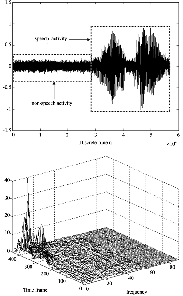
Figure 4. (a) The signal NX[n] composed of N[n] followed by X[n]; (b) Spectrum NX[k] of NX[n].
noise. The spectrum NX[k] of the signal composed of the vacuum noise followed by the noisy speech is shown in Figure 4(b).
3.2. Computing the Average Magnitude of the Noise Spectrum during Non-Speech Activity
The non-speech activity contains 221 time frames with 256 frequency values. After computing the non-speech activity spectrum, we calculate the average of the noise magnitude spectrum for each frequency
 , (5)
, (5)
where E is the average value operator. In the next subsection, we explain the role of μ (k).
3.3. Noise Removal by Subtracting Average Magnitude of Noise Spectrum
The speech activity which is the noisy speech “Real graph” contains 221 rows of time frames and 256 columns of frequency values. The average magnitude of the noise spectrum is subtracted from the noisy speech spectrum resulting in the signal
 . (6)
. (6)
Figure 5 shows the noisy speech frame after subtracting the average noise magnitude spectrum.
3.4. Half-Wave Rectification
In some cases, for each frequency ω, the value of the average magnitude of the noise spectrum is larger than the magnitude of the noisy speech spectrum. This results in negative values after subtracting the average magnitude of the noise spectrum from the noisy speech spectrum. Half-wave rectification consists in replacing those negative values with zero resulting in the signal
 . (7)
. (7)
Figure 6 shows the spectrum of the speech frames after subtracting the average noise magnitude and halfwave rectification.
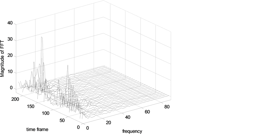
Figure 5. Spectrum of the noisy speech frames after subtracting the average noise magnitude spectrum.
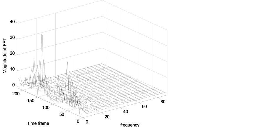
Figure 6. Spectrum of the speech frames after subtracting average noise magnitude and half-wave rectification.
3.5. Reconstruction of the Noisy Speech “Real Graph” Using Inverse Fast Fourier Transform
The flowchart blocks detailed above complete the noise removal algorithm. The conversion from frequency domain to discrete-time domain using the IFFT [7] of the signal ![]() results in the signal
results in the signal ![]() calculated as follows:
calculated as follows:
 . (8)
. (8)
3.6. Transformation of Noisy Speech “Real Graph” in Real Time Using D-to-A Converter
After converting the reconstructed speech signal ![]() from the frequency domain to the discrete time domain using IFFT, the Digital-to-Analog converter transforms
from the frequency domain to the discrete time domain using IFFT, the Digital-to-Analog converter transforms ![]() back to the real-time speech signal
back to the real-time speech signal![]() . We implemented this algorithm using Matlab. The sound corresponding to
. We implemented this algorithm using Matlab. The sound corresponding to ![]() was generated also using Matlab. Successful results were obtained. Noise was effectively reduced from the noisy speech “Real graph”, which confirms the validity of our noise-removal algorithm.
was generated also using Matlab. Successful results were obtained. Noise was effectively reduced from the noisy speech “Real graph”, which confirms the validity of our noise-removal algorithm.
4. Improving the Spectral Subtraction Noise Removal Design
4.1. Frames Averaging
In this section, frames averaging technique was applied in order to improve the performance of the spectral subtraction noise removal design [9] . Frames averaging are represented as an optional step between computing the average magnitude of the noise spectrum and subtracting this average from the magnitude of the noisy speech frames. When applied, frames averaging involve using the magnitude average of several frames of the noisy speech rather than one frame at a time. We limited this research to averaging either three or six consecutive frames. Bigger numbers could result in decreasing in speech intelligibility [6] .
4.2. Varying the Lengths of the Half-Overlapped Data Buffers and Hanning Time Window
In this subsection we investigate the effect that varying the lengths of the half-overlapping data buffer and Hanning time window have on improving the noise removal design. The overlapping of the data buffers was varied between one-half and one-fourth overlapping and the Hanning time window length was varied from 256 points to 128 points and 512 points.
4.3. Statistical Error Analysis
The original algorithm design consisted of no frame averaging with half-overlapped data buffers and 256 points Hanning time windows. Combining those techniques lead to 17 different design configurations shown in Table 1, Table 2, Table 3.
In order to evaluate the improvement in noise removal, we used the Speech to Noise Ratio (SNR) [8] defined as
 , (9)
, (9)

Table 1. Noise removal design using 256 points Hanning window.
Table 2. Noise removal design using 128 points Hanning window.
Table 3. Noise removal design using 512 points Hanning window.
where  is the root-mean-square (RMS) of the reconstructed speech signal
 ![]() after noise removal calculated as follows
after noise removal calculated as follows
 , (10)
and  is the RMS of the vacuum noise N[n] calculated as
 . (11)
We considered as reference SNR (SNRref) the ratio of the RMS of the reconstructed speech signal “Real graph” in Section 3 to the RMS of the vacuum noise. Subsequently, the improvement in noise removal ΔSNR was evaluated by subtracting the SNRref from the SNR of each of the 15 different design configurations in Table 1, Table 2, Table 3 as follows
 . (12)
Improvement indeed occurs whenever ΔSNR is positive. In this application, SNRref was equal to 13.0248 dB, which lead to the ΔSNR values shown in Table 1, Table 2, Table 3.
5. Conclusions
In this research, noise removal from noisy speeches has been studied and analyzed. The study includes methods for removing noise from noisy speeches using spectral subtraction.
Real-time data were sampled using a digital sound recorder system that converted both clean speech “Real graph” and vacuum cleaner noise from analog signals to digital signals at a sampling rate of 44.1 kHz. Noisy speech was digitally generated by corrupting the data of the clean speech “Real graph” with the data of the vacuum cleaner noise. Noise removal in the time domain was not successful. However, in the frequency domain, noise was successfully removed from the noisy speech. Prior to removing noise in the frequency domain, the spectrums of speech and non-speech activities were computed using the FFT of Hanning time-windowed data buffers. Removing noise requires an approximation of the noise during speech activity. The approximation of the noise was obtained by taking the average magnitude of the noise spectrum during non-speech activity. The average magnitude of the noise spectrum during non-speech activity was subtracted from the noisy speech spectrum during speech activity.
Our initial noise removal design consisted of no frame averaging with half-overlapped data buffers and 256 points Hanning time windows. The corresponding reference signal to noise ratio was equal to 13.0248 dB. We then tested a total of 17 modified noise-removal designs in search for the best configuration. Results showed that using any combination of half-overlapped and one-fourth-overlapped data buffers with 128, 256, and 512 points, Hanning windows and three frames or six frames averaging did not improve the performance of the denoising algorithm. However, using one-fourth-overlapped data buffers with 256 points Hanning windows and no frames averaging resulted in the greatest improvement differential SNR in the amount of 0.3371 dB, leading to most noise removal from the noisy speech “Real graph”. Thus we consider that our goal of denoising noisy speech signals has been successfully achieved.
References
- Hymavathy, K.P. and Janardhanan, P. (2013) Noise Filtering in Speech Using Frequency Response Masking Technique. International Journal of Emerging Trends in Engineering and Development, 2.
- Muangjaroen, S. and Yingthawornsuk, T. (2012) A Study of Noise Reduction in Speech Signal Using FIR Filtering. Proceedings of the International Conference on Advances in Electrical and Electronics Engineering, Pattaya, 13-15 April 2012.
- Kumar, T.L. and Rajan, K.S. (2012) Noise Suppression in Speech Signals Using Adaptive Algorithms. International Journal of Engineering Research and Applications, 2, 718-721.
- Aggarwal, R., Singh, J.K., Gupta, V.K., Rathore, S., Tiwari, M. and Khare, A. (2011) Noise Reduction of Speech Signal Using Wavelet Transform with Modified Universal Threshold. International Journal of Computer Applications, 20, 15-19.
- Verteletskaya, E. and Simak, B. (2010) Speech Distortion Minimized Noise Reduction Algorithm. Proceedings of the World Congress on Engineering and Computer Science, Vol. I, San Francisco, 20-22 October 2010.
- Boll, S.F. (1979) Suppression of Acoustic Noise in Speech Using Spectral Subtraction. IEEE Transactions on Acoustic, Speech and Signal Processing, 27, 113-120. http://dx.doi.org/10.1109/TASSP.1979.1163209
- Rabiner, L.R. and Schafer, R.W. (1978) Digital Processing of Speech Signals. Prentice Hall, Upper Saddle River.
- Quantieri, T.F. (2001) Discrete-Time Speech Signal Processing: Principles and Practice. Prentice Hall, Upper Saddle River.
- Allen, J. (1977) Short Term Spectral Analysis, Synthesis, and Modification by Discrete Fourier Transform. IEEE Transactions on Acoustic, Speech and Signal Processing, 25, 235-238. http://dx.doi.org/10.1109/TASSP.1977.1162950