Journal of Signal and Information Processing
Vol. 4 No. 1 (2013) , Article ID: 28273 , 14 pages DOI:10.4236/jsip.2013.41002
Near-Lossless Compression Based on a Full Range Gaussian Markov Random Field Model for 2D Monochrome Images
![]()
1Department of Computer Science and Engineering, Annamalai University, Annamalai Nagar, India; 2Department of Computer Applications, Mailam Engineering College, Mailam, India.
Email: kseethaddeau@gmail.com, rekhavaiyapuri@gmail.com
Received April 23rd, 2012; revised July 5th, 2012; accepted August 21st, 2012
Keywords: Image Compression; FRGMRF Model; Bayesian Approach; Seed Values; Error Model
ABSTRACT
This paper proposes a Full Range Gaussian Markov Random Field (FRGMRF) model for monochrome image compression, where images are assumed to be Gaussian Markov Random Field. The parameters of the model are estimated based on Bayesian approach. The advantage of the proposed model is that it adapts itself according to the nature of the data (image) because it has infinite structure with a finite number of parameters, and so completely avoids the problem of order determination. The proposed model is fitted to reconstruct the image with the use of estimated parameters and seed values. The residual image is computed from the original and the reconstructed images. The proposed FRGMRF model is redefined as an error model to compress the residual image to obtain better quality of the reconstructed image. The parameters of the error model are estimated by employing the Metropolis-Hastings (M-H) algorithm. Then, the error model is fitted to reconstruct the compressed residual image. The Arithmetic coding is employed on seed values, average of the residuals and the model coefficients of both the input and residual images to achieve higher compression ratio. Different types of textured and structured images are considered for experiment to illustrate the efficiency of the proposed model. The results obtained by the FRGMRF model are compared to the JPEG2000. The proposed approach yields higher compression ratio than the JPEG whereas it produces Peak Signal to Noise Ratio (PSNR) with little higher than the JPEG, which is negligible.
1. Introduction
Image content analysis is an important research issue in computer vision because applications such as multimedia, image retrieval through Internet, TV broadcast, and storage management etc. require high speed transmission of data and higher compression ratio with high quality. To fulfil these requirements, the size of the data needs to be compressed. Usually, image compression techniques are categorized into lossy and lossless. The lossy compression techniques concentrate on high compression ratio whereas the lossless compression techniques concentrate on high quality. Both the techniques have disadvantage: The lossy does not maintain high quality while the lossless does not maintain high compression ratio. Most of the image compression techniques come under either dictionary-based schemes or statistical-based approaches. The former is computational and time consuming when compared to the latter. The lossy compression technique is developed based on Discrete Cosine Transform (DCT) and on entropy coding while the lossless compression technique uses predictive coding technique, which also follows entropy coding. The lossless JPEG2000 or JPEG-LS is the current standard for lossless image compression [1-3]. The JPEG2000 is developed based on wavelet transform, scalar or trellis coded quantizer, and arithmetic coder. In JPEG2000, the input image is transformed by wavelet transform and the transform coefficients are put into two groups. Each group consists of blocks in the wavelet domain. The transform coefficients are quantized with the help of scalar or trellis coded quantizer, and then the arithmetic coder is applied to code the coefficients.
Hewlett-Packard developed a coding scheme LOCO-I [4] during the standardization process, which is the base for the current standard of the lossless compression. LOCO-I utilises the features of simple fixed context model and complex context model for capturing higherorder dependencies, which attains compression ratios similar or superior to that of state-of-the-art schemes based on arithmetic coding. Memon and Wu [5] proposed a scheme, CALIC, which is presented as a competitor for the standard; it gives similar or better performance at the increased computational complexity when compared to that of LOCO-I. These schemes are based on the same idea of predicting a pixel value on the basis of the values of adjacent pixels. The simplicitydriven schemes like JPEG standard have some limitations in their compression performance by the first order entropy of the prediction residuals, which do not achieve the total decorrelation of the data [6]. In complexitydriven schemes like LOCO-I [4], CALIC [5], and TMW [7], the compression gains are obtained by adjusting the model carefully to the image compression application. The literature reveals the significance of the gap between the complexity-driven schemes and simplicity-driven schemes. The gap between the two schemes is diminished by FELICS algorithm [8]. FELICS maintains the performance with moderate compression ratio at the expense of low computational complexity.
Most of the compression community people, including those in the medical image processing, feel that instead of approaching in terms of the dichotomy between lossless and lossy, it is better to establish an algorithm, which consists of features of both techniques and also it can be a trade-off between them. It establishes a method to develop near-lossless compression algorithm. Near-lossless means no pixel is changed in magnitude by more than error tolerance gray levels compared to the original pixel [9]. Error tolerance means that the quantity of the difference between the original image and decompressed image is negligible. Though many researchers [9-11] have developed near-lossless compression algorithm based on differential pulse code modulation (DPCM) for continuous-tone images, there is a lack of decreasing the computational time as well as increasing the compression ratio. Chen and Ramabadran [10] proposed a scheme based on DPCM coding and two types of uniform scalar quantizers with less distortion rate. Ke and Marcellin [11] have extended the concept by generalising and incorporating entropy-minimization of the quantized predictor error. It is observed from the literature that most of the algorithms demand more computational effort to attain moderate compression ratio. This motivated us to development the proposed algorithm.
The proposed technique uses the predictive coding based statistical approach. In this approach, after estimating the parameters, the model generates the pixel values within negligible time period. Also there is no dictionary-based data storage overhead. In the proposed technique, very sharp edges are slightly smoothed. But this problem is overcome by estimating the parameters precisely with the help of M-H algorithm as discussed in Sections 4 and 5.
In order to analyse image content, stochastic models like Random Field (RF) [12], Markov Random Field (MRF) [13-16], and Gibbs field (GF) [17,18] are investigated. Moreover, the degree of accuracy of parameter estimation plays a significant role in obtaining satisfactory results in low-level image processing. In earlier works, classical approaches such as Least Square (LS) [13,19] and Maximum Likelihood Estimation (MLE) [15,20] methods were used to estimate the parameters, which were found to be unsatisfactory for reconstructing the images after compression [13,16] or they require some post processing [16,21,22] or iterative procedures [23-25]. Later the Bayesian approach was studied by [26-29] for parameter estimation that could give higher precision. It is also observed from the literature that the emphasis is on parameter estimation, not on identification of the order of the model [30]. The reason for not concentrating on the order determination or model identification is that computational complexity arises as the order increases. Selecting the most suitable model for describing individual time series can improve the performance of the prediction process.
Collopy and Armstrong [31] suggest that there is no single model that performs better than the others in all types of data (images). In [32], the authors emphasize the need for incorporating knowledge into the model selection process by associating image characteristics with the model performance. Later, Arinze [32] proposed the use of learning algorithm for model selection and is adopted in other works [33-35]. The approaches treat the model selection as a classification problem in which a learning algorithm is used as the classifier. This adds more to computational complexity.
In the proposed method, there is no question of model selection and order determination, for it has infinite structure with a finite number of parameters and so completely avoids the problem of order determination [28,29]. The advantage of the present approach is that the number of parameters fixed is only four and the order does not increase the computational complexity, since the estimation of these parameters is the same irrespective of the order of the model, and hence it increases the efficiency of the model. So, the proposed model is more a generalized one for most images.
The rest of the paper is organized as follows: The overview of the proposed work is presented in Section 2. Section 3 discusses the proposed model and its features. In Section 4, the parameter estimation is discussed. The error model and its parameter estimation technique are discussed in Section 5. The measure of performance is presented in Section 6 and the results of the experiments are demonstrated in Section 7. The conclusion is drawn in Section 8.
2. Overview of the Proposed Work
In this paper, a Full Range Guassian Markov Random Field (FRGMRF) model is proposed for image compression. The proposed compression method performs the compression process at two stages: first, the actual input image is performed using FRGMRF model; second, the residual image is performed based on the error model discussed in Section 5. The proposed family of FRGMRF model is completely free from order determination as discussed in the previous Section. An input image  of size L × L is assumed to be a Gaussian Markov Random Field (GMRF), which is segregated into various non-overlapping subimages of equal fixed sizes of M × M where M < L. Using the Bayesian methodology, the parameters of the model are estimated for each subimage as discussed in Section 4. Using the estimated parameters K, α, θ and
 , the coefficients
  of the model are computed. Based on the model coefficients and seed values, the subimage is generated. This process is repeated for the entire image. The reconstructed subimages are synthesised to form the entire image, which is denoted as
 . The residual image
  is computed from the actual input image
  and the reconstructed image
 . With the assumption that the residual image does not have the spatial direction, the proposed FRGMRF model is redefined as an error model as discussed in Section 5. The error model is employed to reconstruct the residual image to maintain good quality. The parameters of the error model are estimated by employing the Metropolis-Hastings (M-H) algorithm. Many iterative algorithms, including Gibbs sampler and Expectation Maximization (EM) algorithm are shown to be special cases of the M-H algorithm. The M-H algorithm needs less than half of the time taken by other iterative techniques [36]. Based on the estimated parameters of the error model and seed values, the compressed image is decompressed. The residual image is computed from the actual residual image and its reconstructed image. The average value of the residual is calculated. Now, the parameters, seed values and the average are stored for each subimage. The arithmetic coding [37,38] is used on the images compressed by the FRGMRF model and the error model to obtain furthermore compression. The stored pixel values, average of the residuals and the coefficients of the error model are utilised to reconstruct the subimages. The reconstructed subimages are grouped together to form the entire image, which is denoted as
 . Again, error image
  is computed from
  and
and . The average is computed on
  and it is stored together with parameters values and seed values. Based on the stored values, the error image is reconstructed. Now, the reconstructed image of actual input and the residual image are added together, which results in the final reconstructed image. The final reconstructed image is almost error free. Various steps involved in the proposed work are demonstrated with a block diagram in Figure 1.
3. Proposed Model
Generally, the pixels in a small image region are linearly dependent. The linear dependency among the pixels is extracted to predict the missing pixels in that region. As illustrated in Figure 2(a), the center pixel X(s) linearly depends on its neighbouring pixels. The properties of the FRGMRF model allow us to define the likelihood function . This facilitates the statistical estimation of the unknown pixel values. As mentioned in Section 1, the LSE and MLE methods are not satisfactory. Hence, in this article, the Bayesian approach is adopted to predict the unknown pixels in the small image region by considering the likelihood function aforesaid, which gives the conditional distribution of the neighbourhood pixels given the original,
  and the prior information obtained from the domain block,
  , where g represents the neighbourhood pixels. The joint posterior distribution
 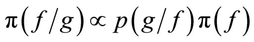 is obtained by using these two components and the Bayes’s theorem. By keeping all these points, a model is proposed as in Equation (1). Let X be a random variable that represents the intensity value of a pixel at location (k, l) in an image of size M ´ M. The random variable X is assumed to be independent and identically distributed (i.i.d.) Gaussian random variables in discrete state space with mean zero and variance σ2, because the noise is independent and identically distributed Gaussian random variable which is incorporated with X. The noise is denoted with the symbol
  and it follows the normal distribution, i.e.
 .
.
Since  is a stochastic process, where
 ,
,  can be considered as a Markov process because it has the conditional probability:
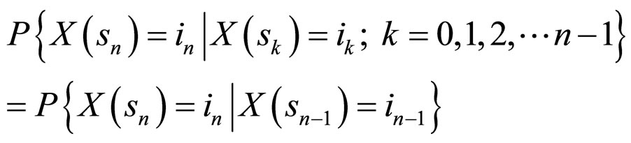
for all ik,  and sk belonging to the state space S and
 .
.
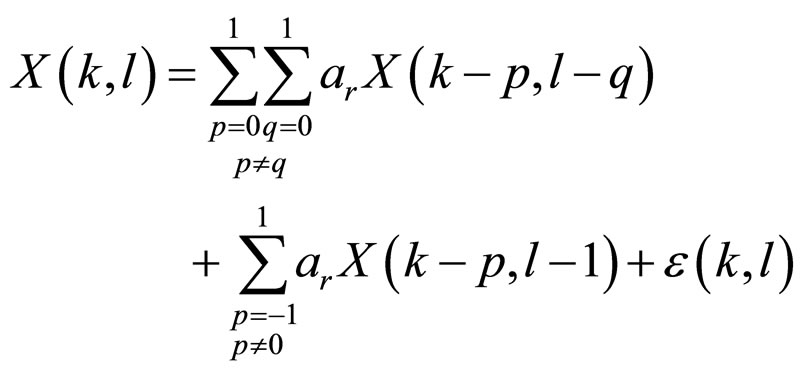
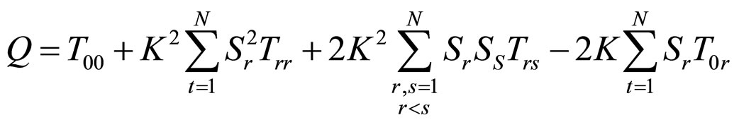
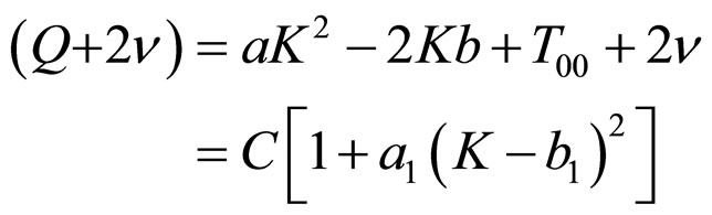
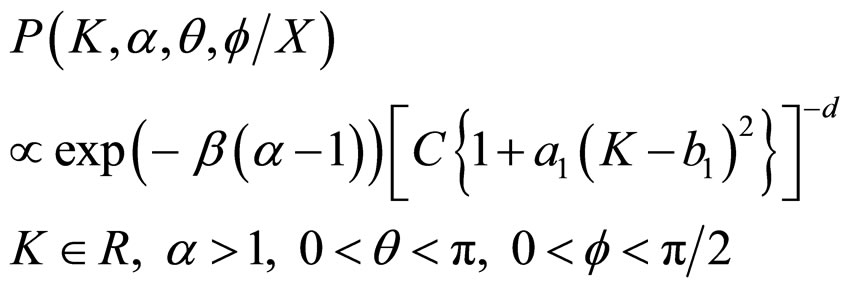
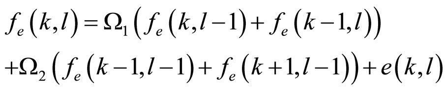
Thus, we propose a model in Equation (1), Full Range Gaussian Markov Random Field (FRGMRF) model,
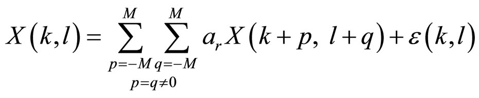 (1)
(1)
where
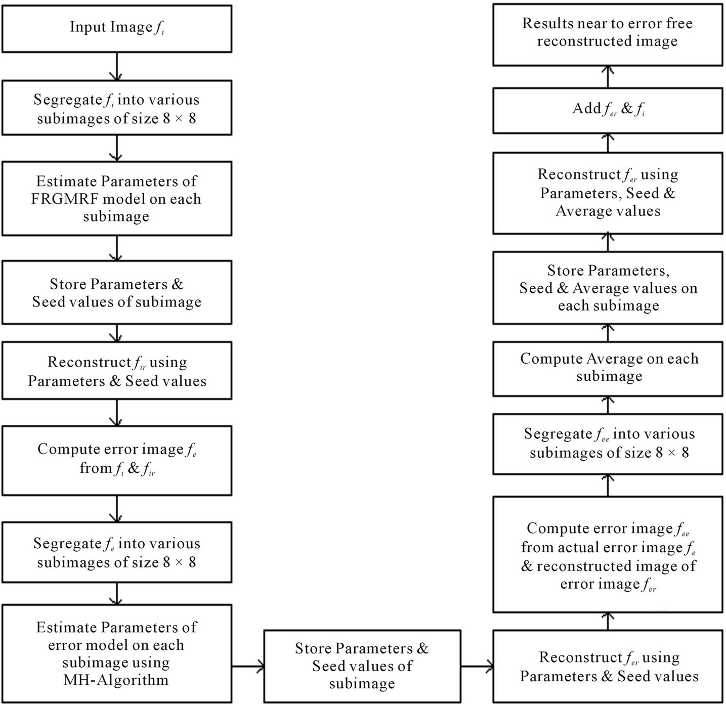
Figure 1. Block diagram of the proposed work.
 (a)
(a)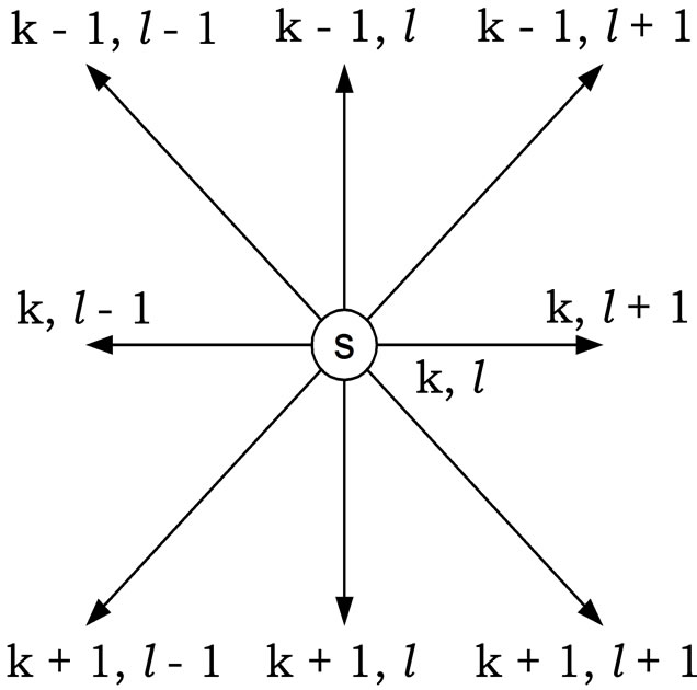 (b)
(b)
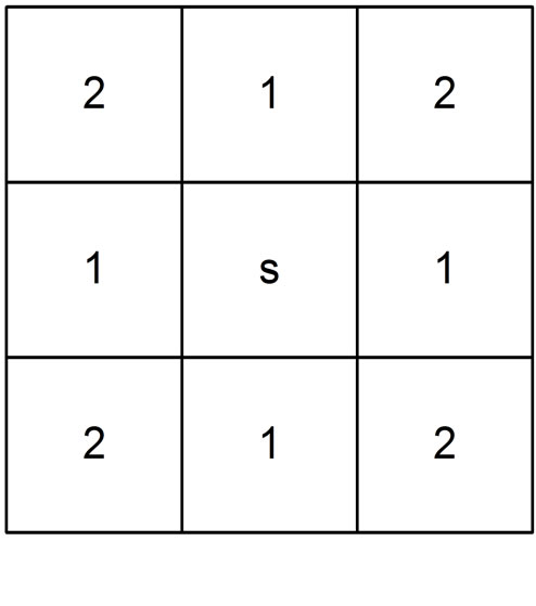
Figure 2. (a) Relationship among neighbour sets; (b) Neighbour sets for different FRGMRF model with orders.
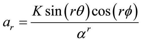
 (1a)
(1a)
and K, α, θ, and f are real parameters. The , model coefficients, which are computed by substituting the model parameters K, α, θ, and f in Equation (1a). The model parameters are interrelated.
The proposed model is employed to analyse a two dimensional discrete gray-scale image. The image is partitioned into various subimages of size M × M, to locally characterize the nature of the image. With the Markovian assumption, the conditional probability of X(s) given all other values only depends upon the nearest neighbourhood values.
The initial assumptions about the parameters are K ∈ R: real value, α > 1, and q, . Some of the models used in the previous works-white noise, Markov model with finite order and infinite order can be regarded as special cases of the proposed model. Thus
1) if we set q = 0, then the FRGMRF model reduces to the white noise process;
2) when α is large, the coefficients ars become negligible as “r” increases. So the FRGMRF model reduces to a Gaussian Markov Random model with order r approximately, for a suitable value of r, where r is the order of the model;
3) when α is chosen to be less than one, then the FRGMRF model becomes an explosive infinite order Gaussian Markov Random model.
The fact that  has regression on its neighbourhood pixels gives rise to the terminology of dependency process. However, in this case the dependence of
  on neighbourhood values may be true to some extent. In fact, the process is Gaussian under the assumption that the
  are Gaussian and in this case its probabilistic structure is completely determined by its second order properties. The second order properties meant for the proposed FRGMRF model is asymptotically stationary up to order two, provided 1 – α < K < α – 1. Finally the range of the parameters of the model is set as with the constraints K ∈ R, α > 1, 0 < q < p, 0 < f < p/2.
The non-causal model proposed in Equation (1) represents the pixel  as a linear combination of nearest neighbourhood values on each side as shown in Figure 2(a), and the influence of the horizontal and vertical pixels on the centre is higher than that of the diagonal pixels. The order of influence of neighbourhood pixels on its centre is illustrated in Figure 2(b).
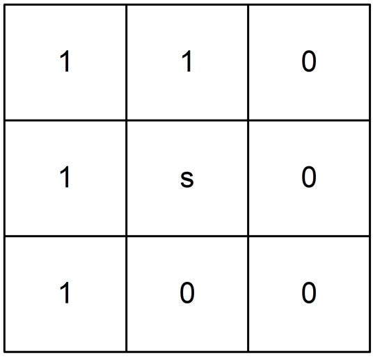
While reconstructing the compressed image, only the previous values viz. upper triangular elements are known and are represented by one, and all the other elements are zero as depicted in Figure 3(b). Hence, the pixel  is predicted by using the upper triangular elements only, which are categorized into two sets according to the order of neighbourhood pixels as shown in Figure 3(a).
Hence, the non-causal model given in Equation (1) is redefined as a causal model, with the combination of two sets of elements as described in Figure 3(a):
 (2)
(2)
where,
 (2a)
(2a)
 (2b)
(2b)
By using the above constraints in Equations (2a) and
 (a)
(a)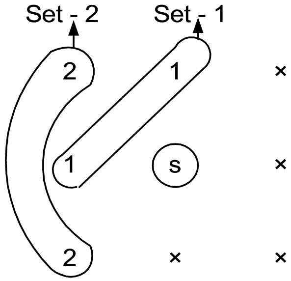 (b)
(b)
Figure 3. (a) Order (priority) of the neighbour sets; (b) 1 represents availability of the pixels; 0 represents nonavailability of the pixels.
(2b), the causal model given in Equation (3) is obtained from Equation (1)
 (3)
(3)
where,
 , and
, and .(3a)
.(3a)
The model given in Equation (3) is used to reconstruct the compressed image data at stage one.
4. Parameter Estimation
In order to implement the proposed FRGMRF model, the parameters are to be estimated. The parameters K, α, θ and f are estimated, by taking the suitable prior information for the hyper parameters b, g, and d, based on Bayesian methodology [28,29]. The hyper parameters are meant for the parameters of the prior distribution of the actual model parameters K, α, θ and f. The hyper parameters, approximately estimated by using the mean and standard deviation of the pixel values of the subimage are to be estimated. Just for the computational purpose, the pixel values of each subimage are arranged as one-dimensional vectors ,
,  (M × M = M2 = N). Since the error term
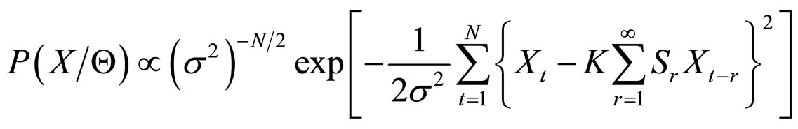
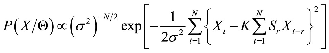
  in Equation (3) is independent and identically distributed Gaussian random variable, the joint probability density function of the stochastic process
  is given by
 (4)
(4)
where, ;
; , and
, and  .
.
When the real data are analyzed with finite number of N observations, the range for the index “r” viz., 1 to ¥, reduces to 1 to N and so the joint probability density function of the observations given in Equation (4); the summation  can be replaced by
  which gives
 (5)
(5)
By expanding the square in the exponent, we get
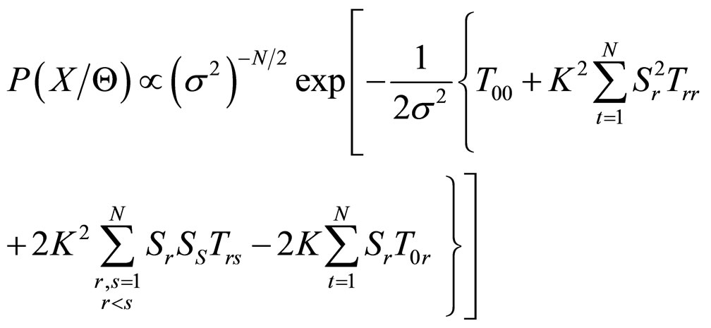 (6)
(6)
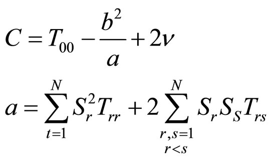
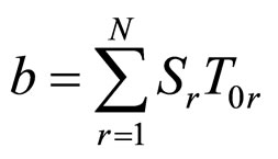
where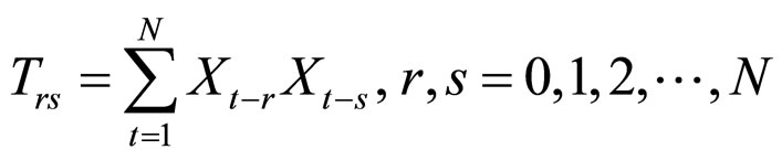 .
.
The above joint probability density function can be written as
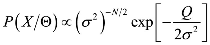 (7)
(7)
where,
 ,
,  ,
,  ,
,  and σ2 > 0.
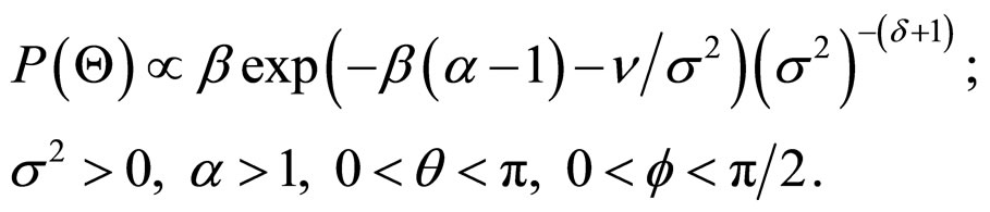
The prior distribution of the parameters is assigned as follows:
1) α is distributed as the displaced exponential distribution with parameter β, i.e.
 (8)
(8)
2) σ2 has the inverted gamma distribution with parameter  and δ, i.e.
 (9)
(9)
3) K, q and f are Uniformly distributed over their domain, i.e. , a constant;
 ,
,  ,
, .
.
So, the joint prior density function of Q is given by
 (10)
(10)
where, P is used as a general notation for the probability density function of the random variables given within the parentheses following P.
Using (7), (10) and Bayes theorem, the joint posterior density of K, α, θ, f and σ2 is obtained as
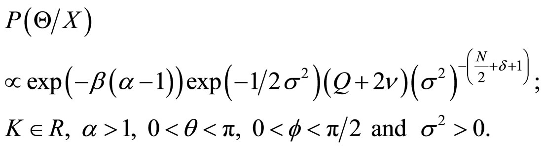 (11)
(11)
Integrating (11) with respect to σ2, the posterior density of K, α, θ and f is obtained as
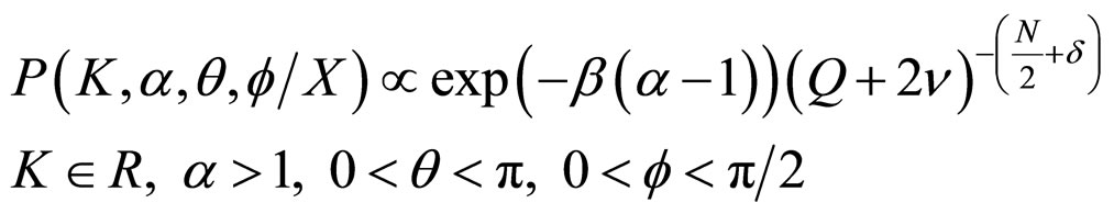 ; (12)
where
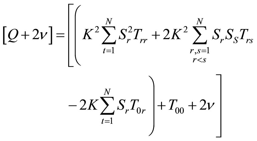 (13)
(13)
That is,
 (14)
(14)
where
 ;
; ;
; 
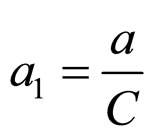
Thus, the above joint posterior density of K, a, q and f can be rewritten as
 (15)
(15)
where, .
.
This shows that, given α, θ and f, the conditional distribution of K is “t” distribution located at b1 with (2d – 1) degrees of freedom (d.f.).
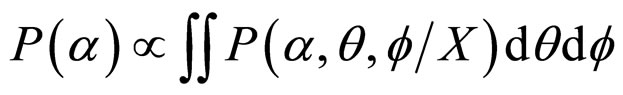
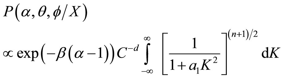
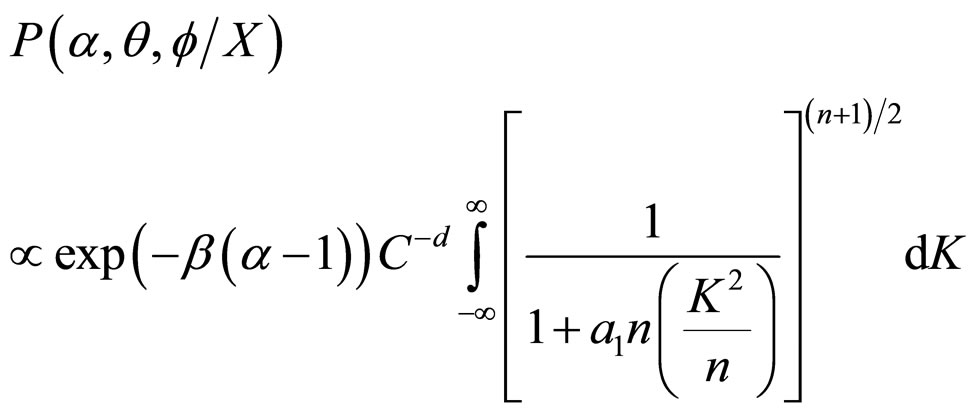
The proper Bayesian inference on K, α, θ and f can be obtained from their respective posterior densities. The joint posterior density of α, θ and f, namely,  , can be obtained by integrating (15) with respect to K.
Thus,
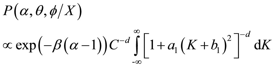 (16)
(16)
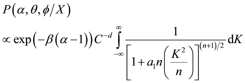
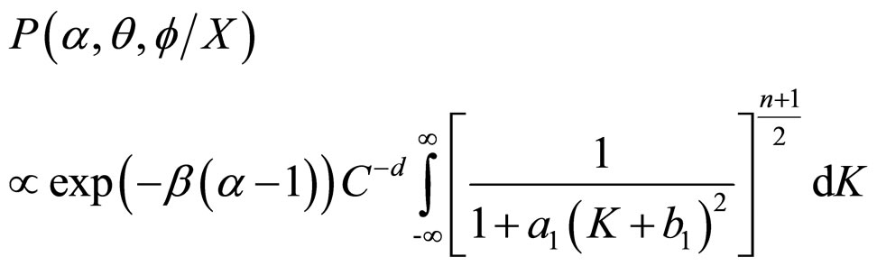 (17)
(17)
where, n = (2d −1) d.f.
Thus, the joint posterior density of α, θ and f is obtained as
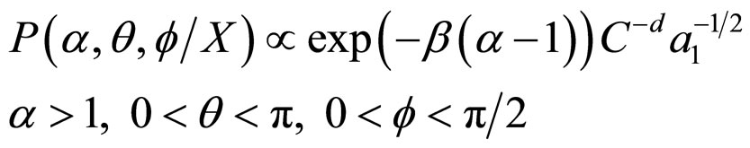 (18)
(18)
The derivation of Equation (18) from Equation (17) is discussed in APPENDIX.
The marginal posterior density of α, θ and f in (18) is a complicated function and is analytically not solvable. Therefore, we can find the original posterior density of α, θ and f numerically from the joint density (18).
That is,
Similarly,
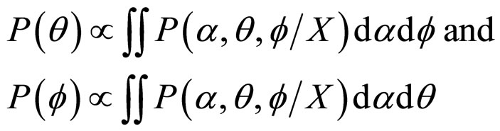 (19)
(19)
The point estimates of the parameters α, θ and f may be taken as the means of the respective marginal posterior distribution i.e. posterior means. With a view to minimize the computations, we first obtain the posterior mean of α numerically. Then fix α at its posterior mean and evaluate the conditional means of θ and f fixing α at its mean. We fix α, θ and f at their posterior means respectively and then evaluate the conditional mean of K.
Thus, the estimates are
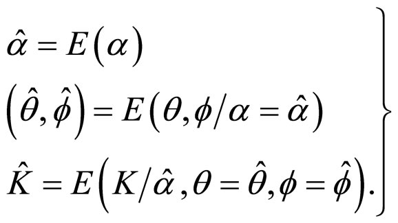 (20)
(20)
The estimated parameters K, α, θ and f are used in Equation (3a) to compute the coefficients  of the model presented in Equation (3) and then the model coefficients are applied in Equation (3) to reconstruct the compressed image.
5. Error Model
The residual image  is computed from the actual input image
  and the reconstructed image
 . Since the residual image
  has no spatial direction among the pixels, the angle θ is set to zero in the proposed model in Equation (1). Now, the proposed FRGMRF model becomes white noise model as in Equation (21), because the first term in Equation (1) becomes zero and the error term, that is, second term only remains.
 (21)
(21)
where ,
,  represents error term, which follows the Markov process [39] and
  are the Markov coefficients.
By applying the constraints used in Equations (2a) and (2b), the model in Equation (21) is reconstructed as stationary second-order MR(2) model as follows:
 (22)
(22)
where  and
and .
.
The Metropolis-Hastings (M-H) algorithm is employed to estimate the coefficients  and
and  of the error model for each subimage. The set of coefficients
  lying in the region
  is calculated and that satisfies the following stationarity conditions.
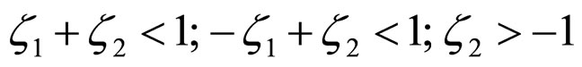 .
.
The computed coefficient values  and
and  are substituted in Equation (22) to obtain the decompressed image.
The following algorithm is employed to estimate the coefficients  and
and .
.
M-H Algorithm
Step 1: Check the stationarity conditions for the set of coefficient values .
.

Step 2: A sample of draws from the posterior distribution of the parameters  can be obtained by successively sampling from
 , where
 .
.
Step 3: Simulate s2 from 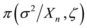 using
using .
.
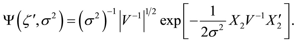
Step 4: Generate candidates from the density function
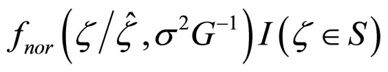
where  is the normal density function,
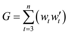 and
and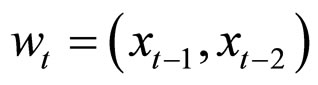 .
.
Step 5: At jth iteration (the current value s2(j)) draws a candidate  from a normal density with mean
  and covariance
 .
.
1) If it satisfies stationarity conditions given in Step 1, then move to this point with probability
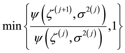
2) Otherwise set .
.
Step 6: Repeat Step: 2 to Step: 5 until it satisfies the condition 1) of Step: 5.
After estimating the parameters  and
and , the model expressed in Equation (22) is employed to reconstruct the compressed subimage.
6. Measures of Performance
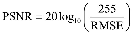
The performance of the proposed FRGMRF model is evaluated by means of Root Mean-Squared Error (RMSE) and Peak Signal to Noise Ratio (PSNR)
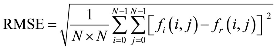
where  and
and  are actual input image and final reconstructed image of size 256 ´ 256 respectively.
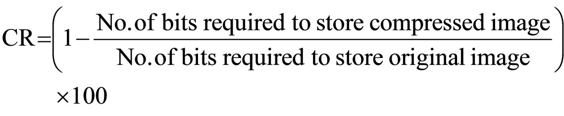
The compression ratio (CR) is calculated in percentage as follows:
7. Experiments and Results
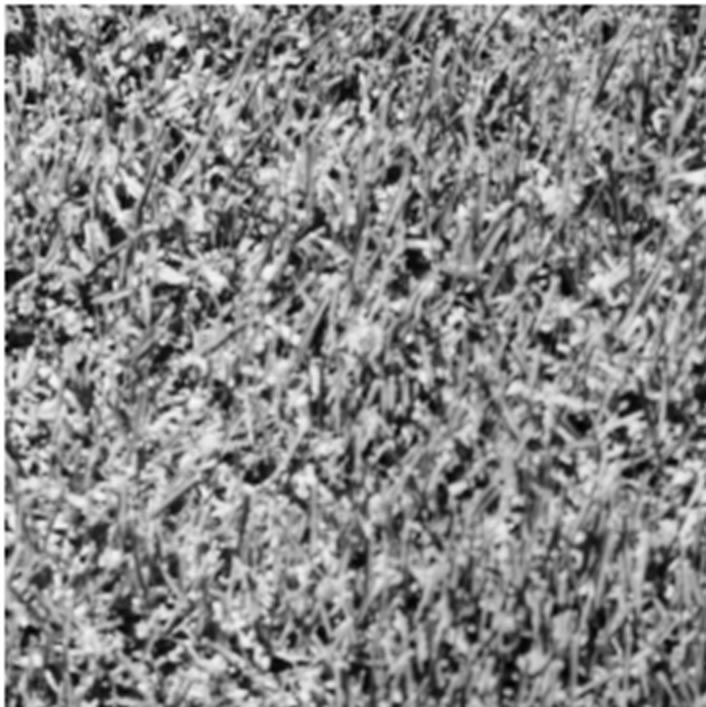
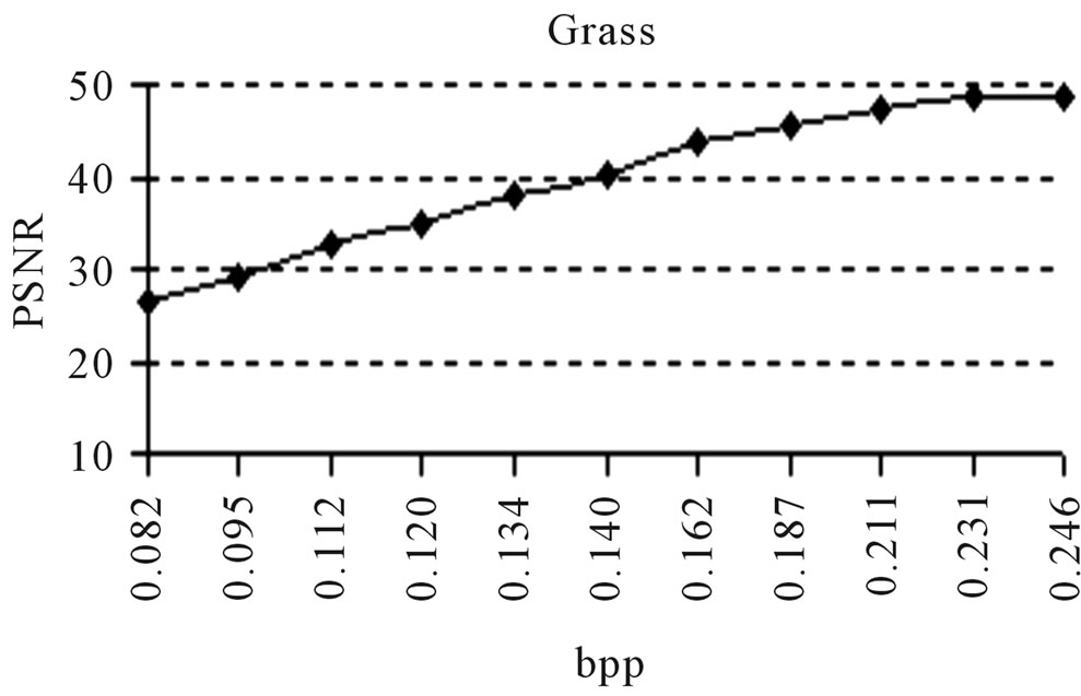
The proposed FRGMRF model and the error model discussed in Section 4 and Section 5 are experimented on different types of monochrome images for compression and decompression. For sample, two standard textured images D9 (Grass) and D29 (Beach-Sand) and a structured image viz. the Barb image, each of size 256 × 256 with pixel values in the range 0 to 255 are given in Figures 4(a)-(c) respectively. The textured images are taken from standard Brodatz album [40]. The input image is divided into various non-overlapping subimages of equal size of 8 × 8. The parameters of the proposed FRGMRF model are estimated for each subimage as discussed in Section 4. Using the estimated parameters, the coefficients of the model are computed. The coefficients and a few pixel values are stored. Based on the model coefficients and pixel values, the subimage is generated. This process is repeated for the entire image. All the reconstructed subimages are grouped together to form the entire image. The reconstructed images by the proposed method, corresponding to the original images shown in Figures 4(a)-(c), are presented in Figures 4(d)-(f) respectively. The proposed image compression scheme is also compared to JPEG2000. The compressed version of the original images for JPEG2000 is obtained with a quality factor 60, by conducting the experiment with Advanced JPEG Compressor V4.8 [41] software, and the outputs corresponding to the images shown in Figures 4(a)-(c) are presented in Figures 4(g)-(i). The compression ratios along with RMSE and PSNR values by the proposed method and the JPEG2000 are presented in Table 1.
Based on the actual input image  and the reconstructed image
 , the residual image
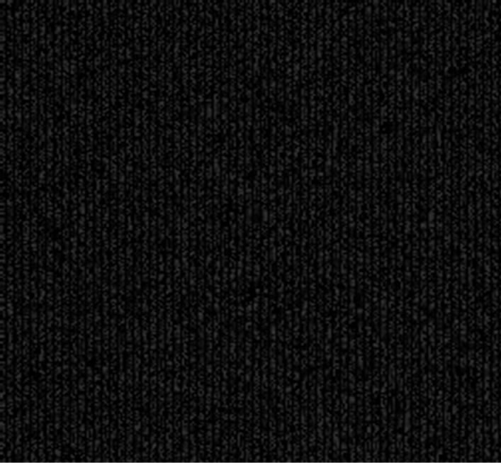
  is computed. The residual images of D9-Grass, D29-Beach-Sand and Barb images are presented in Figures 5(a)-(c) respectively. As discussed in Section 1, the sharp edges are smoothed while reconstructing the compressed images by the FRGMRF model. Smoothed means the loss of information. The information lost (residual image) is extracted by differentiating the images
  and
and . The error model discussed in Section 5 is employed on the residual image to obtain furthermore quality. For more precise estimation of the parameters of the error model, the M-H algorithm discussed in Section 5 is used for accurate prediction of the pixels in the residual image. The procedure used for the actual input image (FRGMRF model) is adopted for the residual image (error model). The arithmetic coding is used on image data compressed by the FRGMRF model and the error model to achieve higher compression ratio. The output of the experiment is presented in Figures 6(d)-(f) and the results obtained are given in Table 2. The outputs are obtained by adding the images generated by the FRGMRF model and error model. The final outputs are compared with the outputs obtained by JPEG2000 with the quality factor 95 and presented in Figures 6(g)-(i). Conducting the experiment at various levels of quality factors and bpp, the final outputs are obtained. From the experiment, it is observed that the quality factor 95 yields good reconstruction quality at different bit rates. The optimum bpp is fixed at
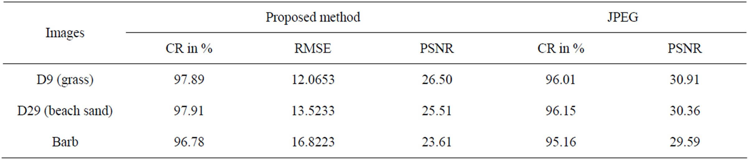
Table 1. Compression results of FRGMRF model and the results obtained by JPEG2000 with quality factor 60.
 (a)
(a)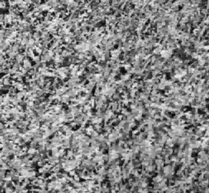 (d)
(d)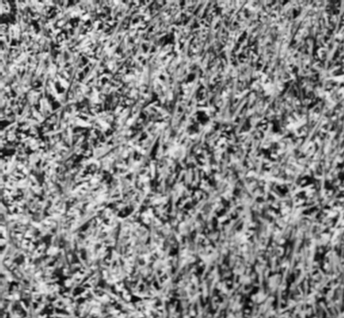 (g)
(g) (b)
(b)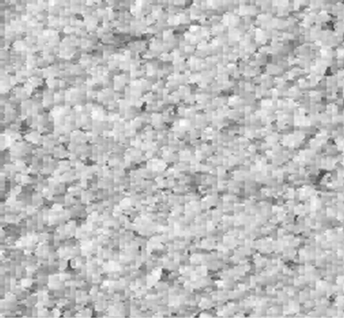 (e)
(e)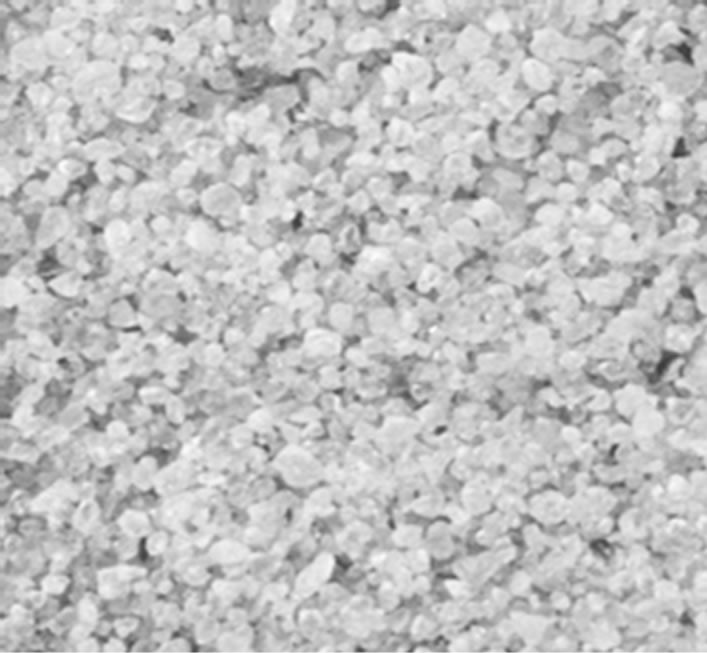 (h)
(h)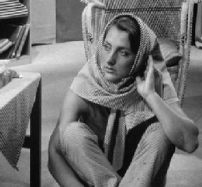 (c)
(c) (f)
(f) (i)
(i)
Figure 4. (a), (b) and (c) are original images; (d), (e) and (f) are reconstructed images by the proposed model; (g), (h) and (i) are reconstructed images by JPEG with quality factor 60.
 (a)
(a)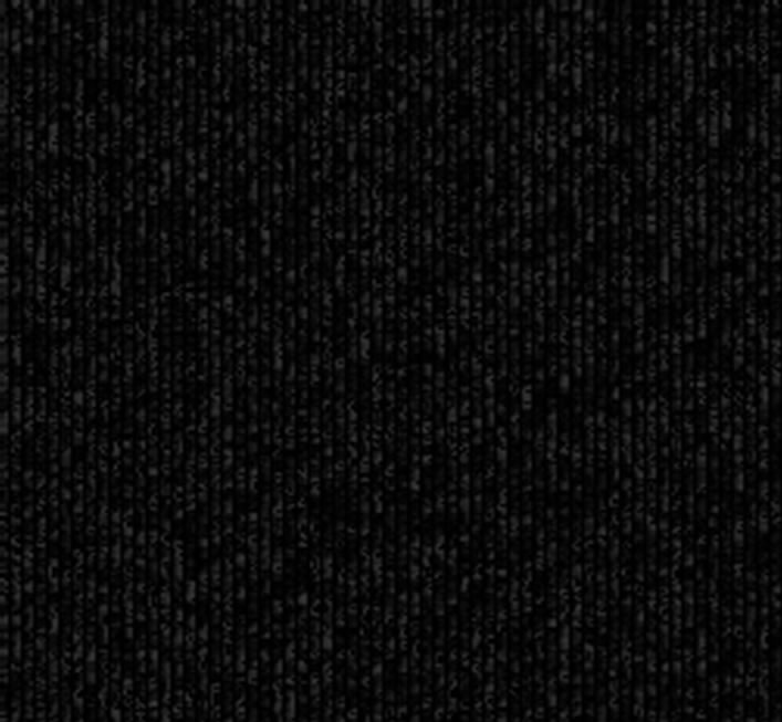 (b)
(b) (c)
(c)
Figure 5. Residual image: (a): D9-grass; (b): D29-beach sand; (c): Barb.
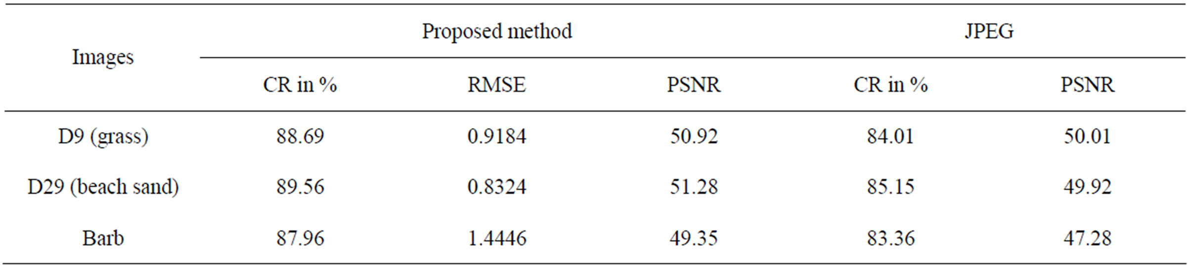
Table 2. Final compression results of combined FRGMRF and ERROR model, and the results obtained by JPEG2000 with quality factor 95.
 (a)
(a)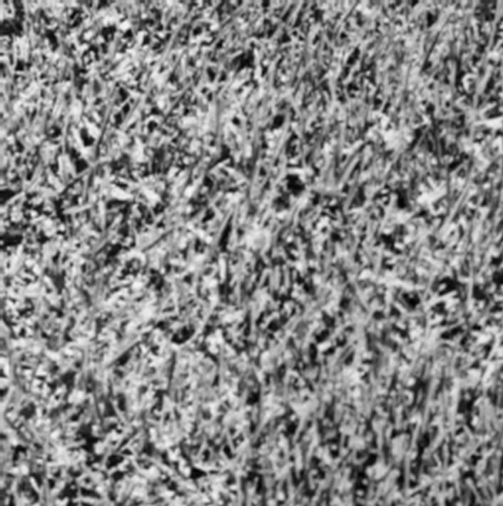 (d)
(d) (g)
(g)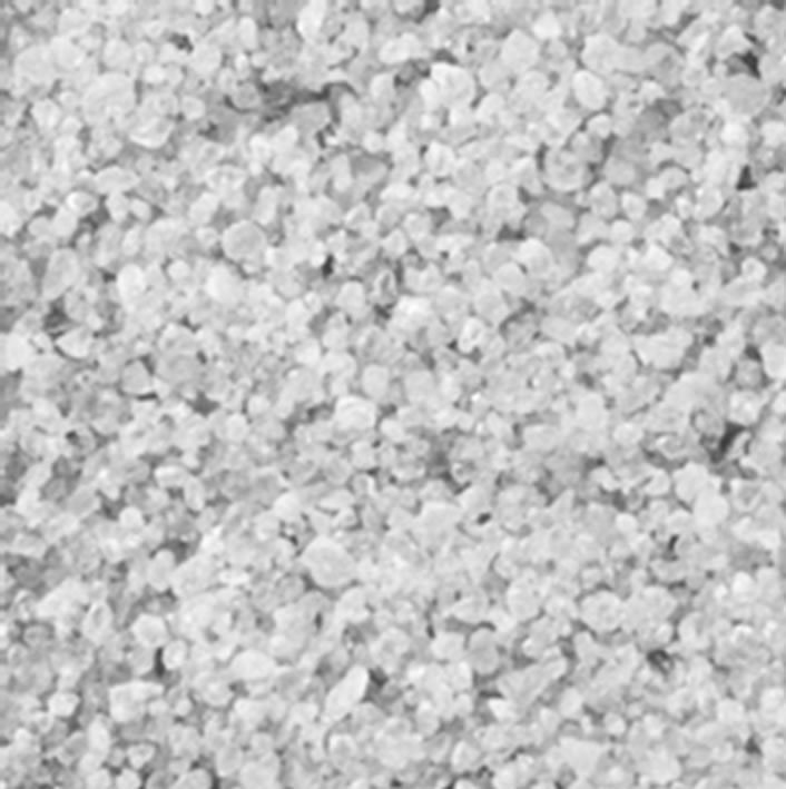 (b)
(b)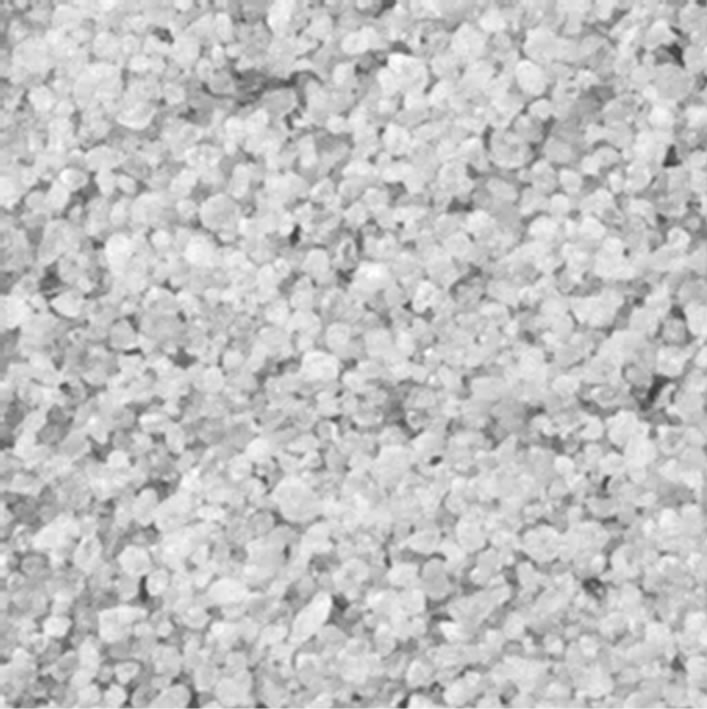 (e)
(e) (h)
(h)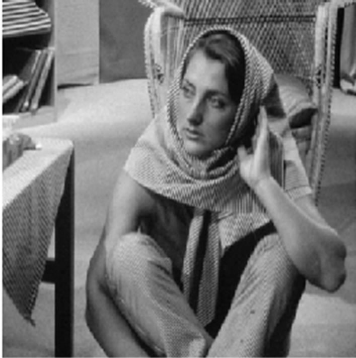 (c)
(c) (f)
(f)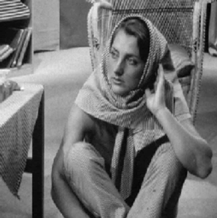 (i)
(i)
Figure 6. (a), (b) and (c) are original images; (d), (e) and (f) are reconstructed images by the proposed model; (g), (h) and (i) are reconstructed images by JPEG with quality factor 95.
0.231 for D9-Grass, 0.232 for D29-Beach-Sand and 0.235 for Barb images. The graphical representations of the outputs obtained by the experiments conducted on D9-Grass, D29-Beach-Sand and Barb images at various PSNR vs. bpp are presented in Figures 7(a)-(c). Next, a comparative study is carried out at different PSNR vs. Quality Factor on the same images. But, due to the space constraint, it is not possible to present all the outputs of the experiment here. The obtained results show that the proposed method requires more or less the same bpp for textured type (Grass and Beach-Sand) images while it produces less PSNR with high bpp for structured (Barb) images. This is illustrated in Figure 7. From the experimental results, it is observed that the proposed method gives higher compression ratio with good reconstruction quality for both textured and structured images.
8. Conclusions and Future Work
In this paper, a family of FRGMRF model and an error model are proposed for monochrome continuous-tone still image compression. Since the residual image  has no spatial direction among the pixels, the angle θ is set to zero in the proposed model in Equation (1). Thus, it facilitates to derive the error model from the proposed FRGMRF model. The parameters of the FRGMRF model are estimated using the Bayesian approach. A few pixel values of each subimage and the coefficients of the model are stored. Using these values, the image is reconstructed and the residual image is computed from the actual input image and the reconstructed image. The error model is fitted on residual image to compress and decompress. The procedure used to compress the actual input image is used on residual image. The arithmetic coding is subjected to store some pixel values, average values and the coefficients of the model computed on actual input image and the residual image to obtain furthermore compression. The performance of the proposed model is measured with standard measures such as PSNR and RMSE, and the outputs are compared with the outputs obtained by JPEG2000 at different quality factors. The results obtained are comparable with the existing methods.
The proposed model can be applied in data mining for clustering, classification, prediction, and searching. In the proposed method, there is no question of model selection and order determination, as it has infinite structure with a finite number of parameters and so completely avoids the problem of order determination. The number of parameters fixed is only four and the order does not increase the computational complexity, since the estimation of these parameters is the same irrespective of the order of the model, and hence it increases the efficiency of the model. So, the proposed model is a
 (a)
(a)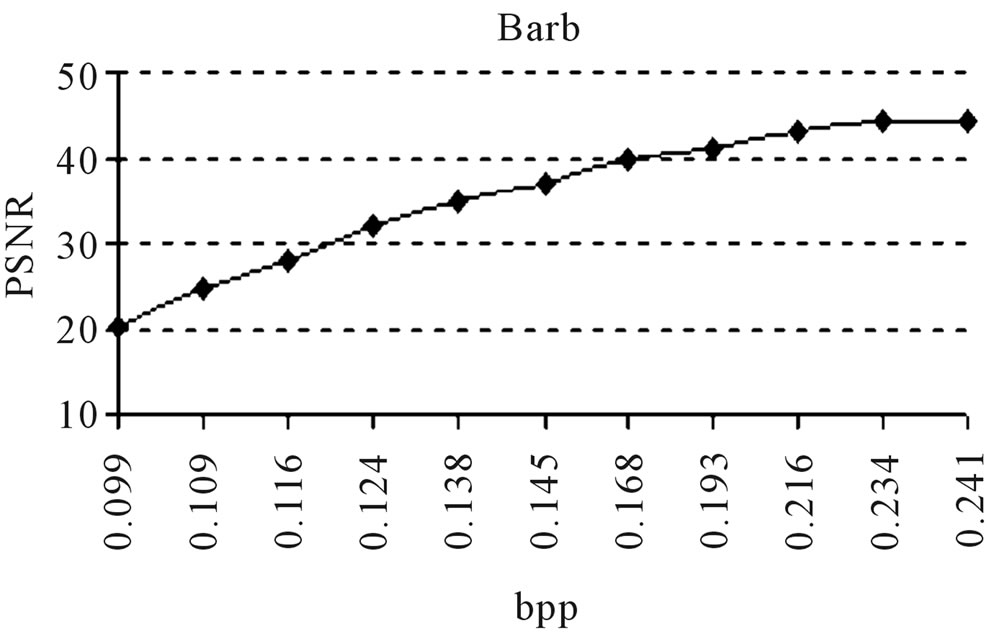 (b)
(b)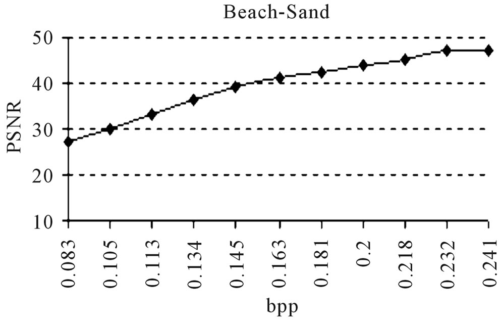 (c)
(c)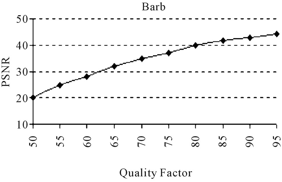 (d)
(d)
Figure 7. (a), (b), (c): Comparison of PSNR vs. bpp; (d): Comparison of PSNR vs. Quality factor.
generalized one for different categories of images. Hence, the proposed model can also be extended to colour image compression by restructuring it as a three dimensional model.
REFERENCES
- M. Rabbani and R. Joshi, “An Overview of the JPEG2000 Still Image Compression Standarad,” Signal Processing: Image Comunication, Vol. 17, No. 1, 2002, pp. 3-48. doi:10.1016/S0923-5965(01)00024-8
- “JPEG-LS: Lossless and Near-Lossless Coding of Continuous-Tone Still Images,” ISO/IEC JTC 1/SC 29/WG 1 FCD 14495, 1997.
- A. P. Morgan, L. T. Watson and R. A. Young, “A Gaussian Derivative Based Version of JPEG for Image Compression and Decompression,” IEEE Transactions on Image Processing, Vol. 7, No. 9, 1998, pp. 1311-1320. doi:10.1109/83.709663
- M. J. Weinberger, G. Seroussi and G. Sapiro, “The LOCO-I Lossless Image Compression Algorithm: Principles and Standardization into JPEG-LS,” IEEE Transactions on Image Processing, Vol. 9, No. 8, 2000, pp. 1309-1323. doi:10.1109/83.855427
- N. Memon and X. Wu, “Context-Based, Adaptive, Lossless Image Coding,” IEEE Transactions on Communications, Vol. 45, No. 4, 1997, pp. 437-444. doi:10.1109/26.585919
- M. Feder and N. Merhav, “Relation between Entropy and Error Probability,” IEEE Transaction on Information Theory, Vol. 40, No. 1, 1994, pp. 259-266. doi:10.1109/18.272494
- M. Meyer and P. Tischer, “TMW—A New Method for Lossless Image Compression,” Proceedings of the International Symposium on Picture Coding, Berlin, September 1997, pp. 120-127.
- P. G. Howard and J. S. Vitter, “Fast and Efficient Lossless Image Compression,” Proceedings of the Data Compression Conference, Snowbird, 30 March-2 April 1999, pp. 351-360.
- S. Yea and W. A. Pearlman, “A Wavelet-Based TwoStage Near-Lossless Coder,” IEEE Transactions on Image Processing, Vol. 15, No. 11, 2006, pp. 3488-3500. doi:10.1109/TIP.2006.877525
- K. Chen and T. V. Ramabadran, “Near-Lossless Compression of Medical Images through Entropy-Coded DCPM,” IEEE Transactions on Medical Image, Vol. 13, No. 3, 1994, pp. 538-548. doi:10.1109/42.310885
- L. Ke and M. M. W. arcellin, “Near-Lossless Image Compression: Minimum-Entropy, Constrained-Error DPCM,” IEEE Transactions on Image Processing, Vol. 7, No. 2, 1998, pp. 225-228. doi:10.1109/83.660999
- R. L. Kashyap, “Univariate and Multivariate Random Field Models for Images,” Computer Graphics and Image Processing, Vol. 12, No. 3, 1980, pp. 257-270. doi:10.1016/0146-664X(80)90014-3
- E. J. Delp, R. L. Kashyap and O. Robert Mitchel, “Image Data Compression Using Autoregressive Time Series Models,” Pattern Recognition, Vol. 11, No. 5-6, 1979, pp. 313-323. doi:10.1016/0031-3203(79)90041-4
- R. Chellappa, S. Chatterjee and R. Bagdazian, “Texture Synthesis and Compression Using Gaussian-Markov Random Field Models,” IEEE Transactions on Systems Man, and Cybernetics, Vol. 15, No. 2, 1985, pp. 298-303. doi:10.1109/TSMC.1985.6313361
- D. K. Panjwani and G. Healey, “Markov Random Field Models for Unsupervised Segmentation of Textured Color Images,” IEEE Tansactions on Pattern and Analsysis and Machine Intelligence, Vol. 17, No. 10, 1995, pp. 939-1014. doi:10.1109/34.464559
- R. G. Aykroyd and S. Zimeras, “Inhomogeneous Prior Models for Image Reconstruction,” Journal of American Statistical Association,” Vol. 94, No. 447, 1999, pp. 934-946. doi:10.1080/01621459.1999.10474198
- B. Cholamond, “An Iterative Gibbsian Technique for Simultaneous Structure Estimation and Reconstruction of Mary Images,” Pattern Recognition, Vol. 22, No. 6, 1989, pp. 747-761. doi:10.1016/0031-3203(89)90011-3
- H. Derin and H. Elliott, “Modelling and Segmentation of Noisy and Textured Images Using Gibbs Random Fields,” IEEE Tansactions on Pattern Analysis and Machine Intelligence, Vol. 9, No. 1, 1987, pp. 39-55. doi:10.1109/TPAMI.1987.4767871
- J. Bennett and A. Khotanzad, “Multispectral Random Field Models for Synthesis and Analysis of Color Images,” IEEE Transactions on Pattern Analysis and Machine Intelligence, Vol. 20, No. 3, 1980, pp. 327-332. doi:10.1109/34.667889
- S. R. Kadaba, S. B. Gelfand and R. L. Kashyap, “Recursive Estimation of Images Using Non-Gaussian Autoregressive Models,” IEEE Transactions on Image Processing, Vol. 7, No. 10, 1998, pp. 1439-1452. doi:10.1109/83.718484
- R. Wilson, H. E. Knutsson and G. H. Granlund, “Anisotropic Nonstationary Image Estimation and Its Applications: Part II—Predictive Image Coding,” IEEE Transaction on Image Communications, Vol. 31, No. 3, 1983, pp. 398-404. doi:10.1109/TCOM.1983.1095831
- J.-L. Chen and A. Kundu, “Unsupervised Segmentation Using Multichannel Decomposition and Hidden Markov Models,” IEEE Transactions on Image Processing, Vol. 4, No. 5, 1995, pp. 603-619. doi:10.1109/83.382495
- C. Clausen and H. Wechler, “Color Image Compression Using PCA and Backpropagation Learning,” Pattern Recognition, Vol. 33, No. 9, 2000 pp. 1555-1560. doi:10.1016/S0031-3203(99)00126-0
- M. L. Comer and J. Edward Delp, “Segmentation of Textured Images Using a Multiresolution Gaussian Autoregressive Model,” IEEE Transactions on Image Processing, Vol. 8, No. 3, 1999, pp. 408-420. doi:10.1109/83.748895
- S. W. Lu and H. Xu, “Textured Image Segmentation Using Autoregressive Model and Artificial Neural Network,” Pattern Recognition, Vol. 28, No. 12, 1995, pp. 1807-1817. doi:10.1016/0031-3203(95)00051-8
- D. M. Higdon, J. E. Bousher, V. E. Johnson, T. G. Turkington, D. R. Gilland and R. J. Jaszezak., “Fully Bayesian Estimation of Gibbs Hyper Parameters for Emission Computed Tomography Data,” IEEE Transcations on Medical Imaging, Vol. 16, 1997, pp. 516-526.
- C. D. Elia, G. Pogi and G. Scarpa, “A Tree-Structured Markov Random Field Model for Bayes Image Segmentation,” IEEE Transactions on Image Processing, Vol. 12, No. 10, 2003, pp. 1259-1273. doi:10.1109/TIP.2003.817257
- K. Seetharaman, “A Block-Oriented Restoration in GrayScale Images Using Full Range Autoregressive Model,” Pattern Recognition, Vol. 45, No. 4, 2012, pp. 1591-1601. doi:10.1016/j.patcog.2011.10.020
- K. Seetharaman and R. Krishnamoorthi, “A Statistical Framework Based on a Family of Full Range Autoregressive Models for Edge Extraction,” Pattern Recognition Letters, Vol. 28, No. 7, 2007, pp. 759-770. doi:10.1016/j.patrec.2006.11.003
- A. Sarkar, K. M. S. Sharma and R. V. Sonka, “A New Approach for Subset 2-D AR Model Identification for Describing Textures,” IEEE Transactions on Image Processing, Vol. 6, No. 3, 1997, pp. 407-413. doi:10.1109/83.557348
- F. Collopy and J. S. Armstrong, “Rule-Based Forecasting: Development and Validation of an Expert Systems Approach to Combining Time Series Extrapolations,” Management Science, Vol. 38, No. 10, 1992, pp. 1394-1414. doi:10.1287/mnsc.38.10.1394
- B. Arinze, “Selecting Appropriate Forecasting Models Using Rule Induction, Omega-Internat,” Journal of Management Science, Vol. 22, No. 6, 1994, pp. 647-658.
- C. H. Chu and D. Widjaja, “Neural Network System for Forecasting Method Selection,” Decision Support Systems, Vol. 12, No. 1, 1994, pp. 13-24. doi:10.1016/0167-9236(94)90071-X
- A. R. Venkatachalan and J. E. Sohl, “An Intelligent Model Selection and Forecasting System,” Journal of Forecast, Vol. 18, No. 3, 1999, pp. 167-180. doi:10.1002/(SICI)1099-131X(199905)18:3<167::AID-FOR715>3.0.CO;2-F
- R. B. C. Prudencio, T. B. Ludermir and F. A. T. De Carvalho, “A Model Symbolic Classifier for Selecting Time Series Models,” Pattern Recognition Letters, Vol. 25, No. 8, 2004, pp. 911-921. doi:10.1016/j.patrec.2004.02.004
- S. Chib and E. Greenberg, “Understanding the Metropolis Hastings Algorithm,” American Statistical Association, Vol. 49, No. 4, 1995, pp. 327-335.
- I. H. Witten, R. M. Neal and J. G. Cleary, “Arithmetic Coding for Data Compression,” Communications of the ACM, Vol. 30, No. 6, 1987, pp. 520-540. doi:10.1145/214762.214771
- M. Nelson and J.-L. Gailly, “The Data Compression Book,” 2nd Edition, BPB Publications, New Delhi, 1996, Chapter 5, pp. 113-133.
- D. Cochrane and G. H. Orcutt, “Application of Least Square Regression to Relationships Containing Autocorrelated Error Terms,” Journal of American Statistical Association, Vol. 44, No. 245, 1949, pp. 32-61.
- P. Brodatz, “Textures: A Photographic Album for Artisters and Designerss,” Dover, New York, 1966.
- WinSoftMagic 4.8, “Advanced JPEG Compressor V4.8: Free Downloadable version,” 1999-2005. www.winsoftmagic.com
- S. C. Gupta and V. K. Kapoor, “Fundamentals of Mathematical Statistics,” 8th Edition, Sultan Chand and Sons, New Delhi, Chapter 14, pp. 14.1-14.3.
Appendix
A.1 Derivation of Equation (18) from Equation (17)
Let us consider the Equation (17) in Section 4.
 (1A)
(1A)
The expression given in Equation (1A) can be written as in Equation (2A), since the term b1 can be ignored. Because b1 represents the location of the variate K, which follows t-distribution.
 (2A)
(2A)
 (3A)
(3A)
 (4A)
(4A)
The probability density function  of t-distribution with
  d.f. satisfies the condition
 (5A)
(5A)
Therefore,
 (6A)
(6A)
Now put,  in Equation (4A)
The limits of “K” and “y” remain the same and differentiate the above equation.
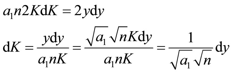
Using these values in Equation (4A) and making use of (6A), we get Equations (7A) and (8A)
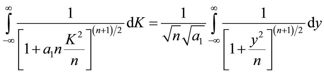 (7A)
(7A)
 (8A)
(8A)
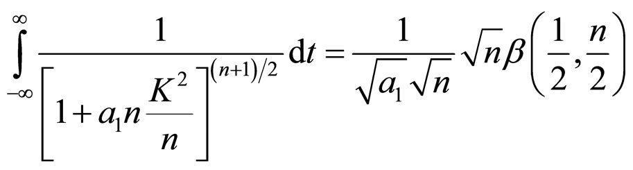
 (9A)
(9A)
The probability density function of Beta distribution of second kind for variate  with
with  d.f. [42] is
 (10A)
(10A)
where  d.f..
d.f..
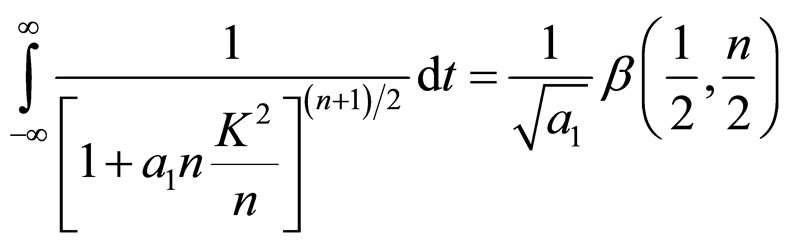
0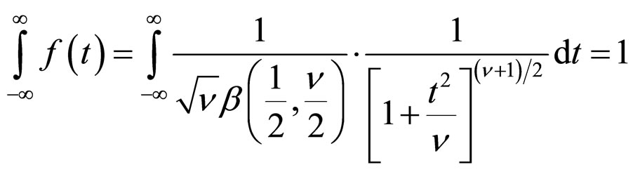 (11A)
(11A)
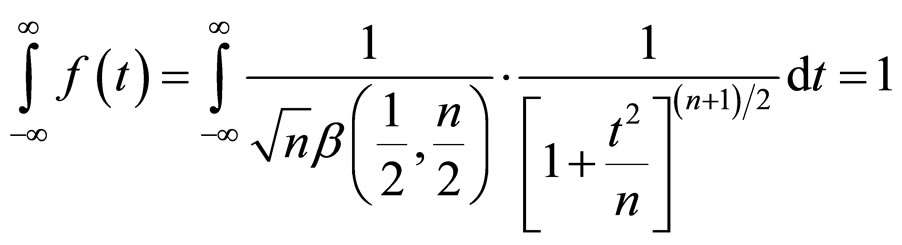
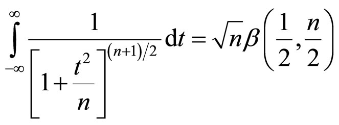
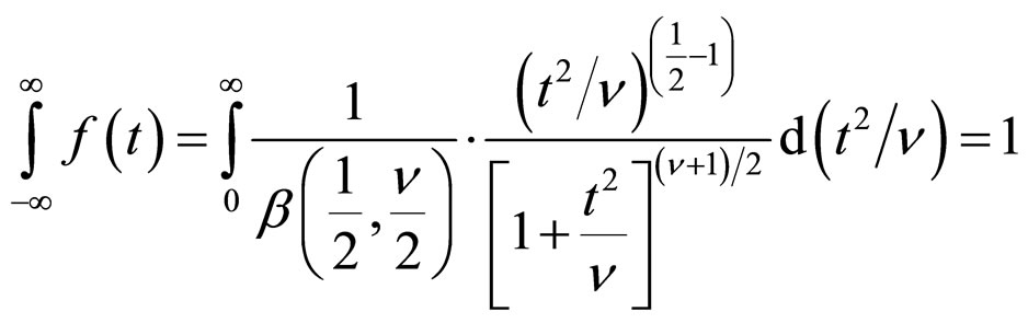
The factor 2 disappearing since the integral form -¥ to ¥ must be unity. The expression in Equation (11A) is the t-distribution with (n–1) d.f..
Acording to Equations (10A) and (11A), the variate
 in Equation (9A) follows t-distribution with n d.f. and its probability density function is equal to 1.
Thus, Equation (9A) can be written as follows:
 (12A)
(12A)
Therefore,
 (13A)
(13A)
As said earlier, the term b1 represents the location of the distribution. So it can be ignored. The expression given in Equation (13A) gives the required result.