Journal of Signal and Information Processing
Vol. 3 No. 2 (2012) , Article ID: 19553 , 8 pages DOI:10.4236/jsip.2012.32019
First and Second Order Statistics Features for Classification of Magnetic Resonance Brain Images
![]()
School of Computer and Systems Sciences, Jawaharlal Nehru University, New Delhi, India.
Email: namita_jnu@rediffmail.com, rkajnu@gmail.com
Received January 10th, 2012; revised February 14th, 2012; accepted March 11th, 2012
Keywords: Alzheimer’s Disease; Magnetic Resonance Imaging; Feature Extraction; Discrete Wavelet Transform; First and Second Order Statistical Features
ABSTRACT
In literature, features based on First and Second Order Statistics that characterizes textures are used for classification of images. Features based on statistics of texture provide far less number of relevant and distinguishable features in comparison to existing methods based on wavelet transformation. In this paper, we investigated performance of texture-based features in comparison to wavelet-based features with commonly used classifiers for the classification of Alzheimer’s disease based on T2-weighted MRI brain image. The performance is evaluated in terms of sensitivity, specificity, accuracy, training and testing time. Experiments are performed on publicly available medical brain images. Experimental results show that the performance with First and Second Order Statistics based features is significantly better in comparison to existing methods based on wavelet transformation in terms of all performance measures for all classifiers.
1. Introduction
Alzheimer’s disease is a form of dementia that causes mental disorder and disturbances in brain functions such as language, memory skills, and perception of reality, time and space. World Health Organization [1] and National Institute on Aging (NIA) [2] highlighted that its early and accurate diagnosis can help in its appropriate treatment. One of the most popular ways of diagnosing Alzheimer by physician is a neuropsychological test like Mini Mental State Examination (MMSE) that test memory and language abilities. But problem with this approach is that it is subjective, human biased and sometimes does not give accurate results [3].
In Alzheimer’s disease, the hippocampus located in the medial temporal lobe of the brain is one of the first regions of the brain to suffer damage [4-6]. The research works [7-10] have found that the rate of volume loss over a certain period of time within the medial temporal lobe is a potential diagnostic marker in Alzheimer’s disease. Moreover, lateral ventricles are on average larger in patients with Alzheimer’s disease. Holodny et al. [11] measured the volume of the lateral ventricles for its diagnosis.
Alzheimer’s Association Neuroimaging Workgroup [12] emphasized image analysis techniques for diagnosing Alzheimer. Among various imaging modalities, Magnetic Resonance Imaging (MRI) is most preferred as it is non-invasive technique with no side effects of rays and suitable for the internal study of human brain which provide better information about soft tissue anatomy. However, there is a huge MRI repository, which makes the task of manual interpretation difficult. Hence, computer aided analysis and diagnosis of MRI brain images have become an important area of research in recent years.
For proper analysis of these images, it is essential to extract a set of discriminative features which provide better classification of MRI images. In literature, various feature extraction methods have been proposed such as Independent Component Analysis [13], Fourier Transform [14], Wavelet Transform [15,16], and Texture based features [17-19]. It is a well-known fact that Fourier transform is useful for extracting frequency contents of a signal however it cannot be use for analyzing accurately both time and frequency contents simultaneously. In order to overcome this, wavelet analysis is proposed which analyze time information accurately with the use of a fixed-size window. With the use of variable sized windows, it captures both low-frequency and high-frequency information accurately.
For the classification of Alzheimer’s disease, Chaplot et al. [15] used Daubechies-4 wavelet of level 2 for the extraction of features from MRI. Dahshan et al. [16]
pointed out that the features extracted using Daubechies- 4 Wavelet were too large and may not be suitable for the classification. The research work used Haar Wavelet of level 3 for feature extraction and further reduced features using Principal Component Analysis (PCA) [20] before classification. Though PCA reduce the dimension of feature vector, but it has following disadvantages: 1) Interpretation of results obtained by transformed feature vector become the non-trivial task which limits their usability; 2) The scatter matrix, which is maximized in PCA transformation, not only maximizes between-class scatter that is useful for classification, but also maximizes within-class scatter that is not desirable for classification; 3) PCA transformation requires huge computation time for high dimensional datasets.
In literature [17,18] features based on First and Second Order Statistics that characterizes textures are also used for classification of images. Features based on statistics of texture gives far less number of relevant, non-redundant, interpretable and distinguishable features in comparison to features extracted using DWT. Motivated by this, in our proposed method, we use First and Second Order Statistics for feature extraction. In this paper, we investigated performance of First and Second order based features in comparison to wavelet-based features. Since, the classification accuracy of a decision system also depends on the choice of a classifier. We have used most commonly and widely used classifiers for the classification of MRI brain images. The performance is evaluated in terms of sensitivity, specificity, accuracy, training and testing Time.
The rest of the paper is organized as follows. A brief description of wavelet transform and First and Second order statistics are discussed in Sections 2 and 3 respectively. It is followed by Section 4 which includes experimental setup and results. Finally conclusion and future directions are included in Section 5.
2. Wavelet Transform
The feature extraction stage is one of the important components in any pattern recognition system. The performance of a classifier depends directly on the choice of feature extraction and feature selection method employed on the data. The feature extraction stage is designed to obtain a compact, non-redundant and meaningful representation of observations. It is achieved by removing redundant and irrelevant information from the data. These features are used by the classifier to classify the data. It is assumed that a classifier that uses smaller and relevant features will provide better accuracy and require less memory, which is desirable for any real time system. Besides increasing accuracy, the feature extraction also improves the computational speed of the classifier.
In literature, many feature extraction techniques for images i.e. Fourier transform, Discrete Cosine Transform, Wavelet Transform and Texture based features are proposed. The Fourier transform provides representation of an image based only on its frequency content over the analysis window. Hence, this representation is not spatially localized. In order to achieve space localization, it is necessary for the space window to be short, therefore compromising frequency localization. Wavelets are mathematical functions that decompose data into different frequency components and then study each component with a resolution matched to its scale. Wavelet provides a more flexible way of analyzing both space and frequency contents by allowing the use of variable sized windows. Hence, Wavelet Transform provides better representation of an image for feature extraction [21].
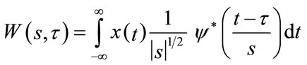
The Continuous Wavelet Transform (CWT) of a signal x(t) is calculated by continuously shifting a scalable wavelet function  and is defined as
 (1)
(1)
where s and  are scale and translation coefficients respectively.
Discrete Wavelet Transform (DWT) is derived from CWT which is suitable for the analysis of images. Its advantage is that discrete set of scales and shifts are used which provides sufficient information and offers high reduction in computation time [21]. The scale parameter (s) is discretized on a logarithmic grid. The translation parameter  is then discretized with respect to the scale parameter. The discretized scale and translation parameters are given by,
  and
and , where m and n are positive integers. Thus, the family of wavelet functions is represented by
 (2)
(2)
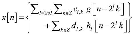
The DWT decomposes a signal x[n] into an approximation (low-frequency) components and detail (high frequency) components using wavelet function and scaling functions to perform multi-resolution analysis, and is given as [21]
 (3)
(3)
where ci,k, i = 1 I are wavelet coefficients and di,k , i = 1
 I are scaling coefficients.
The wavelet and the scaling coefficients are given by
 (4)
(4)
 (5)
(5)
where gi[n – 2ik] and hI[n – 2Ik] represent the discrete wavelets and scaling sequences respectively.
The DWT for a two dimensional image x[m, n] can be similarly defined for each dimension separately. This allows an image I to decompose into a pyramidal structure with approximation component (Ia) and detailed components (Ih, Iv and Id) [22]. The image I in terms of first level approximation component and detailed components is given by
 (6)
(6)
If the process is repeated up to N levels, the image I can be written in terms of Nth approximation component ( ) and detailed components as
 (7)
(7)
Figure 1 shows the process of an image I being decomposed into approximate and detailed components up to level 3. As the level of decomposition is increased, compact but coarser approximation of the image is obtained. Thus, wavelets provide a simple hierarchical framework for better interpretation of the image information [23].
Mother wavelet is the compressed and localized basis of a wavelet transform. Chaplot et al. [15] employed level 2 decomposition on MRI brain images using Daubechies-4 mother wavelet and constructed 4761 dimensional feature vector from approximation part for the classification of two types of MRI brain images i.e. image from AD patients and normal person. Dahshan et al. [16] pointed out that the number of features extracted using Daubechies-4 wavelet were too large and may not be suitable for the classification. In their proposed method, they extracted 1024 features using level 3 decomposition of image using Haar Wavelet and further reduced features using PCA. Though PCA reduce the dimension of feature vector, but it has following disadvantages: 1)
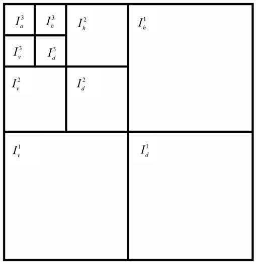
Figure 1. Pyramidal structure of DWT up to level 3.
Interpretation of results obtained by transformed feature vector become the non-trivial task which limits their usability; 2) The scatter matrix, which is maximized in PCA transformation, not only maximizes between-class scatter that is useful for classification, but also maximizes within-class scatter that is not desirable for classification; 3) PCA transformation requires huge computation time for high dimensional datasets.
Hence, there is need to construct a smaller set of features which are relevant, non-redundant, interpretable and helps in distinguishing two or more kinds of MRI images. This will also improve the performance of decision system in terms of computation time. In literature [17,18], First and Second Order Statistics based features are constructed which provide a smaller set of relevant and non-redundant features for texture classification.
3. Features Based on First and Second Order Statistics
The texture of an image region is determined by the way the gray levels are distributed over the pixels in the region. Although there is no clear definition of “texture” in literature, often it describes an image looks by fine or coarse, smooth or irregular, homogeneous or inhomogeneous etc. The features are described to quantify properties of an image region by exploiting space relations underlying the gray-level distribution of a given image.
3.1. First-Order Statistics
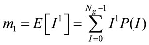
Let random variable I represents the gray levels of image region. The first-order histogram P(I) is defined as:
 (8)
(8)
Based on the definition of P(I), the Mean m1 and Central Moments µk of I are given by
 (9)
(9)
 (10)
(10)
where Ng is the number of possible gray levels.
The most frequently used central moments are Variance, Skewness and Kurtosis given by µ2, µ3, and µ4 respectively. The Variance is a measure of the histogram width that measures the deviation of gray levels from the Mean. Skewness is a measure of the degree of histogram asymmetry around the Mean and Kurtosis is a measure of the histogram sharpness.
3.2. Second-Order Statistics
The features generated from the first-order statistics provide information related to the gray-level distribution of the image. However they do not give any information about the relative positions of the various gray levels within the image. These features will not be able to measure whether all low-value gray levels are positioned together, or they are interchanged with the high-value gray levels. An occurrence of some gray-level configuration can be described by a matrix of relative frequencies Pθ,d(I1, I2). It describes how frequently two pixels with gray-levels I1, I2 appear in the window separated by a distance d in direction θ. The information can be extracted from the co-occurrence matrix that measures second-order image statistics [17,24], where the pixels are considered in pairs. The co-occurrence matrix is a function of two parameters: relative distance measured in pixel numbers (d) and their relative orientation θ. The orientation θ is quantized in four directions that represent horizontal, diagonal, vertical and anti-diagonal by 0˚, 45˚, 90˚ and 135˚ respectively.
Non-normalized frequencies of co-occurrence matrix as functions of distance, d and angle 0˚, 45˚, 90˚ and 135˚ can be represented respectively as
 (11.1)
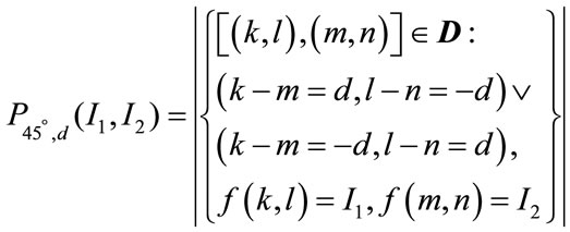 (11.2)
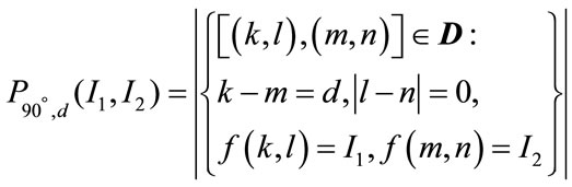 (11.3)
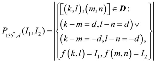 (11.4)
where  refers to cardinality of set, f(k, l) is intensity at pixel position (k, l) in the image of order
  and the order of matrix D is
  .
.
Using Co-occurrence matrix, features can be defined which quantifies coarseness, smoothness and texture— related information that have high discriminatory power.
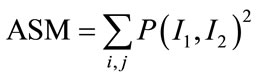
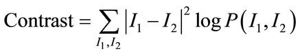
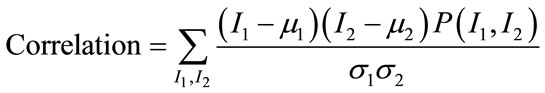
Among them [17], Angular Second Moment (ASM), Contrast, Correlation, Homogeneity and Entropy are few such measures which are given by:
 (12)
(12)
 (13)
(13)
 (14)
(14)
 (15)
(15)
 (16)
(16)
ASM is a feature that measures the smoothness of the image. The less smooth the region is, the more uniformly distributed P(I1, I2) and the lower will be the value of ASM. Contrast is a measure of local level variations which takes high values for image of high contrast. Correlation is a measure of correlation between pixels in two different directions. Homogeneity is a measure that takes high values for low-contrast images. Entropy is a measure of randomness and takes low values for smooth images. Together all these features provide high discriminative power to distinguish two different kind of images.
All features are functions of the distance d and the orientation θ. Thus, if an image is rotated, the values of the features will be different. In practice, for each d the resulting values for the four directions are averaged out. This will generate features that will be rotations invariant.
4. Experimental Setup and Results
In this section, we investigate different combination of feature extraction methods and classifiers for the classification of two different types of MRI images i.e. Normal image and Alzheimer image. The feature extraction methods under investigations are: Features based on First and second order statistics (FSStat), Features using Daubechies-4 (Db4) as described by Chaplot et al. [15] and Haar in combination with PCA (HaarPCA) as described by Dahshan et al. [16]. We will explore the classifiers used by Chaplot et al. [15] (SVM with linear (SVM-L), polynomial kernel (SVM-P) and radial kernel (SVM-R)), Dahshan et al. [16] (K-nearest neighbor (KNN) and Levenberg-Marquardt Neural Classifier (LMNC)) and C4.5. The polynomial kernel of SVM is used with degrees 2, 3, 4 & 5 and best results obtained in terms of accuracy are reported. Similarly radial kernel (SVM-R) is used with various parameters 10i where I = 0 6 and only results corresponding to highest Accuracy is reported. Description of LMNC and remaining classifiers can be found in [25] and [26] respectively.
Textural features of an image are represented in terms of four first order statistics (Mean, Variance, Skewness, Kurtosis) and five-second order statistics (Angular second moment, Contrast, Correlation, Homogeneity, Entropy). Since, second order statistics are functions of the distance d and the orientation , hence, for each second order measure, the mean and range of the resulting values from the four directions are calculated. Thus, the number of features extracted using first and second order statistics are 14.
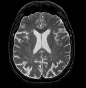
To evaluate the performance, we have considered medical images from Harvard Medical School website [27]. All normal and disease (Alzheimer) MRI images are axial and T2-weighted of 256 × 256 size. For our study, we have considered a total of 60 trans-axial image slices (30 belonging to Normal brain and 30 belonging to brain suffering from Alzheimer’s disease). The research works [7-10] have found that the rate of volume loss over a certain period of time within the medial temporal lobe is a potential diagnostic marker in Alzheimer disease. Moreover lateral ventricles are on average larger in patients with Alzheimer’s disease. Hence, only those axial sections of the brain in which lateral ventricles are clearly seen are considered in our dataset for experiment. As temporal lobe and lateral ventricles are closely spaced, our axial samples thus cover hippocampus and temporal lobe area sufficiently, which can be good markers to distinguish two types of images. Figure 2 shows the difference in lateral ventricles portion between a normal and an abnormal (Alzheimer) image.
In literature, various performance measures have been suggested to evaluate the learning models. Among them the most popular performance measures are following: 1) Sensitivity, 2) Specificity and 3) Accuracy.
Sensitivity (True positive fraction/recall) is the proportion of actual positives which are predicted positive. Mathematically, Sensitivity can be defined as
 (17)
(17)
Specificity (True negative fraction) is the proportion of
 (a)
(a) (b)
(b)
Figure 2. Pyramidal structure of DWT up to level 3.
actual negatives which are predicted negative. It can be defined as
 (18)
(18)
Accuracy is the probability to correctly identify individuals. i.e. it is the proportion of true results, either true positive or true negative. It is computed as
 (19)
(19)
where TP: correctly classified positive cases, TN: correctly classified negative cases, FP: incorrectly classified negative cases and FN: incorrectly classified positive cases.
In general, sensitivity indicates, how well model identifies positive cases and specificity measures how well it identifies the negative cases. Whereas accuracy is expected to measure how well it identifies both categories. Thus if both sensitivity and specificity are high (low), accuracy will be high (low). However if any one of the measures, sensitivity or specificity is high and other is low, then accuracy will be biased towards one of them. Hence, accuracy alone cannot be a good performance measure. It is observed that both Chaplot et al. [15] and Dahshan et al. [16] used highly imbalance data whose classification accuracy was highly biased towards one. Hence, we have constructed balanced dataset (samples of both classes are in same proportion) so that classification accuracy is not biased. Two other performance measures used are training and testing time of learning model.
The dataset was arbitrarily divided into a training set consisting of 12 samples and a test set of 48 samples. The experiment is performed 100 times for each setting and average sensitivity, specificity, accuracy, training and testing time are reported in Table 1. The best results achieved for each classifier corresponding to different performance measure is shown in bold. All experiments were carried out using Pentium 4 machine, with 1.5 GB RAM and a processor speed of 1.5 GHz. The programs were developed using MATLAB Version 7 using combination of Image Processing Toolbox, Wavelet Toolbox and Prtools [28] and run under Windows XP environment.
We can observe the following from Table 1:
1) The classification accuracy with FSStat is significantly more in comparison to both Db4 [15] and HaarPCA [16] for all classifiers.
2) Similar variation in observation is noticed with performance measure sensitivity.
3) For specificity, FSStat provide better results, except for classifiers SVC-P and LMNC, in comparison to both Db4 and HaarPCA.
4) The difference between sensitivity and specificity is
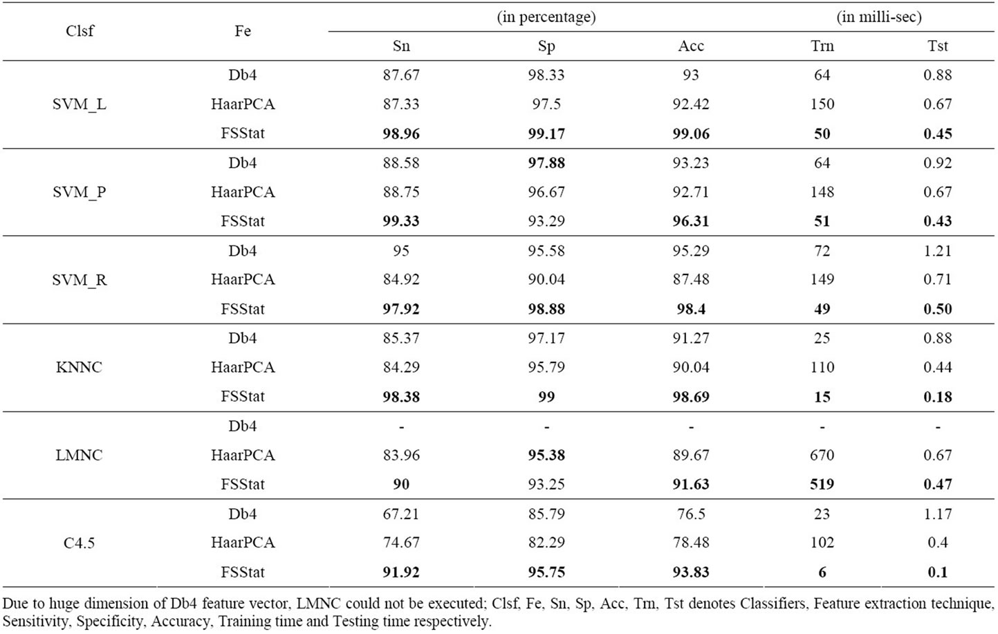
Table 1. Comparison of performance measures values for each combination of feature extraction technique and classifier.
large for both Db4 and HaarPCA in comparison to FSStat. Accuracy obtained using both Db4 and HaarPCA is more even though the sensitivity is low and specificity is high which suggest that classification accuracy obtained is biased.
5) The variation in classification accuracy with different classifiers is not significant with FSStat in comparison with both Db4 and HaarPCA.
6) The training time with FSStat is significantly less in comparison to both Db4 and HaarPCA. This is because the number of features obtained with FSStat is less and does not involve any computation intensive transformation like PCA in HaarPCA.
7) Testing time of an image is not significant in comparison to training time. However, testing time of an image is least with FSStat in comparison to both Db4 and HaarPCA.
From above, it can be observed that the performance of decision system using FSStat is significantly better in terms of all measures considered in our experiment.
5. Conclusions and Future Work
In this paper, we investigated features based on First and Second Order Statistics (FSStat) that gives far less number of distinguishable features in comparison to features extracted using DWT for classification of MRI images.
Since, the classification accuracy of a pattern recognition system not only depends on features extraction method but also on the choice of classifier. Hence, we investigated performance of FSStat based features in comparison to wavelet-based features with commonly used classifiers for the classification of MRI brain images. The performance is evaluated in terms of sensitivity, specificity, classification accuracy, training and testing time.
For all classifiers, the classification accuracy and sensitivity with textural features is significantly more in comparison to both wavelet-based feature extraction techniques suggested in literature. Moreover it is found that FSStat features are not biased towards either sensitivity or specificity. Their training and testing time are also significantly less than other feature extraction techniques suggested in literature. This is because First and Second Order Statistics gives far less number of relevant and distinguishable features and does not involve in computational intensive transformation in comparison to method proposed in literature.
In future, the performance of our proposed approach can be evaluated on other disease MRI images to evaluate its efficacy. We can also explore some feature extraction/construction techniques which provide invariant and minimal number of relevant features to distinguish two or more different kinds of MRI.
REFERENCES
- WHO, “Priority Medicines for Europe and the World,” World Health Organization, 2005.
- NIH, “Progress Report on Alzheimer’s Disease 2004- 2005,” National Institutes of Health (NIH), Bethesda, 2005.
- D. S. Knopman, S. T. DeKosky, J. L. Cummings, H. Chui, J. Corey-Bloom, N. Relkin, G. W. Small, B. Miller and J. C. Stevens, “Practice Parameter: Diagnosis of Dementia (an Evidence-Based Review): Report of the Quality Standards Subcommittee of the American Academy of Neurology,” Neurology, Vol. 56, 2001, pp. 1143-1153. doi:10.1212/WNL.56.9.1143
- C. M. Bottino, C. C. Castro, R. L. Gomes, C. A. Buchpiguel, R. L. Marchetti and M. R. Neto, “Volumetric MRI Measurements Can Differentiate Alzheimer’s Disease, Mild Cognitive Impairment, and Normal Aging,” International Psychogeriatric, Vol. 14, No. 1, 2002, pp. 59-72. doi:10.1017/S1041610202008281
- K. M. Gosche, J. A. Mortimer, C. D. Smith, W. R. Markesbery and D. A. Snowdon, “Hippocampal Volume As an Index of Alzheimer Neuropathology: Findings from the Nun Study,” Neurology, Vol. 58, No. 10, 2002, pp. 1476-1482. doi:10.1212/WNL.58.10.1476
- L. A. Van de Pol, A. Hensel, W. M. Van der Flier, P. Visser, Y. A. Pijnenburg, F. Barkhof, H. J. Gertz and P. Scheltens, “Hippocampal Atrophy on MRI in Frontotemporal Lobar Degeneration and Alzheimer’s Disease,” Journal of Neurology, Neurosurgery & Psychiatry, Vol. 77, No. 4, 2006, pp. 439-442. doi:10.1136/jnnp.2005.075341
- A. George, M. D. Leon, J. Golomb, A. Kluger and A. Convit, “Imaging the Brain in Dementia: Expensive and Futile?” American Journal of Neuroradiology, Vol. 18, 1997, pp. 1847-1850.
- M. P. Laakso, G. B. Frisoni, M. Kononen, M. Mikkonen, A. Beltramello, C. Geroldi, A. Bianchetti, M. Trabucchi, H. Soininen and H. J. Aronen, “Hippocampus and Entorhinal Cortex in Frontotemporal Dementia and Alzheimer’s Disease: A Morphometric MRI Study,” Biological Psychiatry, Vol. 47, No. 12, 2000, pp. 1056-1063. doi:10.1016/S0006-3223(99)00306-6
- M. J. De Leon, J. Golomb, A. E. George, A. Convit, C. Y. Tarshish, T. McRae, S. De Santi, G. Smith, S. H. Ferris and M. Noz, “The Radiologic Prediction of Alzheimer’s Disease: The Atrophic Hippocampal Formation,” American Journal of Neuroradiology, Vol. 14, 1993, pp. 897- 906.
- T. Erkinjuntti, D. H. Lee, F. Gao, R. Steenhuis, M. Eliasziw, R. Fry, H. Merskey and V. C. Hachinski, “Temporal Lobe Atrophy on Magnetic Resonance Imaging in the Diagnosis of Early Alzheimer’s Disease,” Archives of Neurology, Vol. 50, 1993, pp. 305-310. doi:10.1001/archneur.1993.00540030069017
- A. I. Holodny, R. Waxman, A. E. George, H. Rusinek, A. J. Kalnin and M. de Leon, “MR Differential Diagnosis of Normal-Pressure Hydrocephalus and Alzheimer Disease: Significance of Perihippocampal Fissures,” American Journal of Neuroradiology, Vol. 19, No. 5, 1998, pp. 813-819.
- M. Albert, C. DeCarli, S. DeKosky, M. De Leon, N. L. Foster, N. Fox, et al., “The Use of MRI and PET for Clinical Diagnosis of Dementia and Investigation of Cognitive Impairment: A Consensus Report, Prepared by the Neuroimaging Work Group of the Alzheimer’s Association,” 2004.
- C. H. Mortiz, V. M. Haughton, D. Cordes, M. Quigley and M. E. Meyerand, “Whole-Brain Functional MR Imaging Activation from Finger Tapping Task Examined with Independent Component Analysis,” American Journal of Neuroradiology, Vol. 21, No. 9, 2000, pp. 1629- 1635.
- R. N. Bracewell, “The Fourier Transform and Its Applications,” 3rd Edition, McGraw-Hill, New York, 1999.
- S. Chaplot, L. M. Patnaik and N. R. Jagannathan, “Classification of Magnetic Resonance Brain Images Using Wavelets as Input to Support Vector Machine and Neural Network,” Biomedical Signal Processing and Control, Vol. 1, No. 1, 2006, pp. 86-92. doi:10.1016/j.bspc.2006.05.002
- E.-S. A. Dahshan, T. Hosny and A.-B. M. Salem, “A Hybrid Technique for Automatic MRI Brain Images Classification,” Digital Signal Processing, Vol. 20, No. 2, 2010, pp. 433-441. doi:10.1016/j.dsp.2009.07.002
- R. M. Haralick, K. Shanmugan and I. Dinstein, “Textural Features for Image Classification,” IEEE Transactions on Systems: Man, and Cybernetics SMC, Vol. 3, 1973, pp. 610- 621. doi:10.1109/TSMC.1973.4309314
- A. Materka and M. Strzeleck, “Texture Analysis Methods —A Review,” Institute of Electronics, Technical University of Lodz, Brussels, 1998.
- R. K. Begg, M. Palaniswami and B. Owen, “Support Vector Machines for Automated Gait Classification,” IEEE Transactions on Biomedical Engineering, Vol. 52, No. 5, 2005, pp. 828-838. doi:10.1109/TBME.2005.845241
- I. T. Jolliffe, “Principal Component Analysis,” SpringerVerlag, New York, 1986.
- S. G. Mallat, “A Theory of Multiresolution Signal Decomposition: The Wavelet Representation,” IEEE Transactions on Pattern Analysis and Machine Intelligence, Vol. 11, No. 7, 1980, pp. 674-693. doi:10.1109/34.192463
- R. C. Gonzalez and R. E. Woods, “Wavelet and Multiresolution Processing,” In: Digital Image Processing, 2nd Edition, Pearson Education, Upper Saddle River, 2004, pp. 349-408.
- J. Koenderink, “The Structure of Images,” Biological Cybernetics, Vol. 50, No. 5, 1984, pp. 363-370. doi:10.1007/BF00336961
- R. A. Lerski, K. Straughan, L. R. Schad, D. Boyce, S. Bluml and I. Zuna, “MR Image Texture Analysis—An approach to Tissue Characterization,” Magnetic Resonance Imaging, Vol. 11, No. 6, 1993, pp. 873-887. doi:10.1016/0730-725X(93)90205-R
- S. Haykin, “Neural Networks: A Comprehensive Foundation,” Prentice Hall, Upper Saddle River, 1999.
- R. O. Duda, P. E. Hart and D. G. Stork, “Pattern Classification,” Wiley, New York, 2001.
- K. A. Johnson and J. A. Becker, “The Whole Brain Atlas,” 1995. http://www.med.harvard.edu/aanlib/home.html
- R. Duin, P. Juszcak, P. Paclik, E. Pekalska, D. De Ridder and D. Tax, “Prtools, a Matlab Toolbox for Pattern Recognition,” Delft University of Technology, 2004. http://www.prtools.org.