Journal of Data Analysis and Information Processing
Vol.2 No.2(2014), Article ID:46380,11 pages
DOI:10.4236/jdaip.2014.22007
Time Series Modelling with Application to Tanzania Inflation Data
Edward Ngailo1, Eliab Luvanda2, Estomih S. Massawe3*
1Dares Salaam University College of Education, Dares Salaam, Tanzania
2Department of Economics, University of Dares Salaam, Dares Salaam, Tanzania
3Department of Mathematics, University of Dares Salaam, Dares Salaam, Tanzania
Email: *estomihmassawe@yahoo.com
Copyright © 2014 by authors and Scientific Research Publishing Inc.
This work is licensed under the Creative Commons Attribution International License (CC BY).
http://creativecommons.org/licenses/by/4.0/


Received 18 March 2014; revised 20 April 2014; accepted 11 May 2014
ABSTRACT
In this paper, time series modelling is examined with a special application to modelling inflation data in Tanzania. In particular the theory of univariate non linear time series analysis is explored and applied to the inflation data spanning from January 1997 to December 2010. Time series models namely, the autoregressive conditional heteroscedastic (ARCH) (with their extensions to the generalized autoregressive conditional heteroscedasticity ARCH (GARCH)) models are fitted to the data. The stages in the model building namely, identification, estimation and checking have been explored and applied to the data. The best fitting model is selected based on how well the model captures the stochastic variation in the data (goodness of fit). The goodness of fit is assessed through the Akaike Information Criteria (AIC), Bayesian Information Criteria (BIC) and minimum standard error (MSE). Based on minimum AIC and BIC values, the best fit GARCH models tend to be GARCH(1,1) and GARCH(1,2). After estimation of the parameters of selected models, a series of diagnostic and forecast accuracy test are performed. Having satisfied with all the model assumptions, GARCH(1,1) model is found to be the best model for forecasting. Based on the selected model, twelve months inflation rates of Tanzania are forecasted in sample period (that is from January 2010 to December 2010). From the results, it is observed that the forecasted series are close to the actual data series.
Keywords:Time Series, Inflation, Autoregressive

1. Introduction
The concept of time series is based on the historical observations. It involves explaining past observations in order to try to predict those in the future [1] . A time series is a collection of observations measured sequentially through time. These measurements may be made continuously through time or be taken at a discrete set of time points [2] .
Inflation as described by [3] is the persistent increase in the level of consumer prices or persistent decline in the purchasing power of money. Inflation can also be expressed as a situation where the demand for goods and services exceeds their supply in the economy [4] . In reality inflation means that your money can not buy as much as what it could have bought yesterday.
In recent years, inflation has become one of the major economic challenges facing most countries in the world especially those in Africa including Tanzania. Inflation is a major focus of economic policy worldwide as described by [5] . Inflation dynamics and evolution can be studied using a stochastic modelling approach that captures the time dependent structure embedded in the time series inflation data. The autoregressive conditional heteroscedasticity (ARCH) models, with its extension to generalized autoregressive conditional heteroscedasticity (GARCH) models as introduced by [6] and [7] respectively accommodate the dynamics of conditional heteroscedasticity (the changing variance nature of the data). Heteroscedasticity affects the accuracy of forecast confidence limits and thus has to be handled properly by constructing appropriate non-constant variance models [8] .
The most common way of measuring inflation is the consumer price index (CPI) over
monthly, quarterly or yearly. The inflation rate
 at time
 is calculated as

where
 is the current average price level of an economic
basket of goods and services;
is the current average price level of an economic
basket of goods and services;
 is the average price level of the basket a
year ago.
is the average price level of the basket a
year ago.
Within time series modelling, there are two approaches available for forecasting: the univariate and multivariate. In particular this paper will forecast future values of inflation time series data using the univariate forecasting approach, in which forecasts depend only on present and past values of a single series being forecasted.
2. Conditional Heteroscedasticity: Arch-Garch Models
Let
 be the mean-corrected return or rate of inflation,
 be the Gaussian white noise with zero mean
and unit variance and
be the Gaussian white noise with zero mean
and unit variance and
 be the information set at time
 given by
 . Then according
to Engle [6] , the process
. Then according
to Engle [6] , the process
 is ARCH
 if
if

where
 is the standard deviation and
 (1)
(1)
 (2)
(2)
and the error term
 is such that
 (3)
(3)
 (4)
(4)
with non-negativity condition that
 and
and
 for all

The ARCH (1) model is a particular case of the general ARCH model given by
 (5)
(5)
with non-negativity condition that
 and
and .
.
 and
and
 are unknown parameters.
Forecasting with the ARCH Model
The ARCH models provide good estimates of the series before it is realized. Let
 be an observed time series. Then the l-step ahead forecast, for
 at the origin
 , denoted by
 , is taken to
be the minimum mean squared error prediction, that is
, is taken to
be the minimum mean squared error prediction, that is
 minimizes
 where
where
 is a function of the observations. Then according to [9] ,
 (6)
(6)
The forecasts for the
 series do not provide helpful information. It is therefore more useful to consider
the squared returns
series do not provide helpful information. It is therefore more useful to consider
the squared returns
 given by

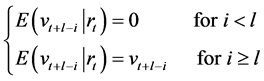
[10] . The l-step ahead forecast for the
 is given by
 (7)
(7)
The obvious possible problem in using the ARCH formulation is that the approach
can lead to a highly parametric model if the
 is large. This necessitates the use of the GARCH model as an extension to the ARCH
model.
is large. This necessitates the use of the GARCH model as an extension to the ARCH
model.
3. The GARCH Model
A process
 is GARCH
 if
if

 (8)
(8)
where
 and
and
 are polynomials in the backshift operator given by


with the restrictions

 and
and
 for
for
 and
and
 being imposed in order to have the conditional variance remaining positive. Equation
(8) can be expressed as
being imposed in order to have the conditional variance remaining positive. Equation
(8) can be expressed as
 (9)
(9)
The GARCH model does not show autocorrelation in the return series
 . However the squared
returns show autocorrelation even though the returns are not correlated. Writing
. However the squared
returns show autocorrelation even though the returns are not correlated. Writing
 in terms of
 yields
 (10)
(10)
Let . Then
 (11)
(11)
where
 for
for
 and
and
 for
for . Thus the equation of
 has an autoregressive moving average ARMA
 representation.
In order to find the GARCH process, we consider solving for
 in Equation (8) and let the variance of
 be
be , getting
 . (12)
Substituting Equation (12) into the Equation (11) one gets
 (13)
(13)
Therefore
 (14)
(14)
Multiplying both sides of Equation (14) by
 and taking expectations we get

But

and since
 is a martingale difference, also
 for
for

Thus the autocovariance of the squared returns for the GARCH model is given by
 (15)
(15)
Dividing both sides of Equation (15) by
 gives the autocorrelation function at
 as
as
 . (16)
Letting
 to denote the
 partial autocorrelation for
 , Equation (16) can
be written as
, Equation (16) can
be written as
 (17)
(17)
By Equation (17),
 cuts off after
 for an ARCH
 process such that
 for
for
 and
and for
for . This is identical to the partial ACF (PACF)
for an AR
. This is identical to the partial ACF (PACF)
for an AR process and decays exponentially [11] .
Assuming
 and
and
 are known, the conditional maximum likelihood estimates of the GARCH Model can be
obtained by maximizing the conditional log-likelihood given by
are known, the conditional maximum likelihood estimates of the GARCH Model can be
obtained by maximizing the conditional log-likelihood given by

with
 and
and

Forecasting with GARCH(p,q) Models
The l-step ahead forecast of the conditional variance in a GARCH model is given by
 (18)
(18)
where
 for
for
 is given recursively by
4. Data Analysis
This section is dedicated to fitting the GARCH family of models to the Tanzania inflation rate data which we obtained from the Tanzania National Bureau of Statistics. The original data set consist of 168 monthly observations of the Tanzania inflation rates spanning from January 1997 to December 2010 as shown in Table 1.
4.1. Pre-Estimation Analysis
To avoid the difficulties of possible premature convergence we perform a pre-fit analysis. This will lead to selecting the appropriate model that adequately describes the data. In this pre-estimation or pre-fit analysis, data are loaded in the form of a price series, and then converted to a return series (stabilized series). The pre-fit analysis checks the return series for correlation and then quantifies the correlation. Because GARCH modelling assumes a return series, we need to convert inflation data (raw data) to returns. Figure 1 below displays raw data of inflation rate and Figure 2 displays the return series converted from the raw.
The returns appear to be quite stable over time and the transformations from Inflation rate data to returns has produced a stationary time series. The GARCH model assumes that return series is a stationary process. This may seem limiting, but the inflation data to return transformation is common and generally guarantees a stable data set for GARCH modelling.
According to [6] any autocorrelations in the series have to be removed before a
GARCH model is constructed. This is done by regressing the squares of the series
 on its past squared values
 with the number of lags determined by the form of the ACF and PACF. The figures
below display the sample autocorrelation function (ACF) of the returns based on
the assumption that all autocorrelations are zero beyond lag zero.
with the number of lags determined by the form of the ACF and PACF. The figures
below display the sample autocorrelation function (ACF) of the returns based on
the assumption that all autocorrelations are zero beyond lag zero.
In Figure 3 and Figure 4, the ACF and PACF provide no indication of the correlation characteristics of the returns. The ACF of squared returns in Figure 5 shows significant correlation and die out slowly. These results indicate that the variance of returns series is conditional on its past history and may change over time.
Statistical test for heteroscedasticity is carried out in order to establish the
presence of ARCH effects in the data. This is shown in
Table 2, Table 3 and
Table 4. This is done using Ljung-Box-Pierce
 and Engle’s ARCH test ([6] [12] ).

Table 1. Summary for statistics for Tanzania’s monthly inflation.
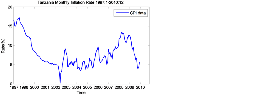
Figure 1. Time plot of monthly inflation in Tanzania.
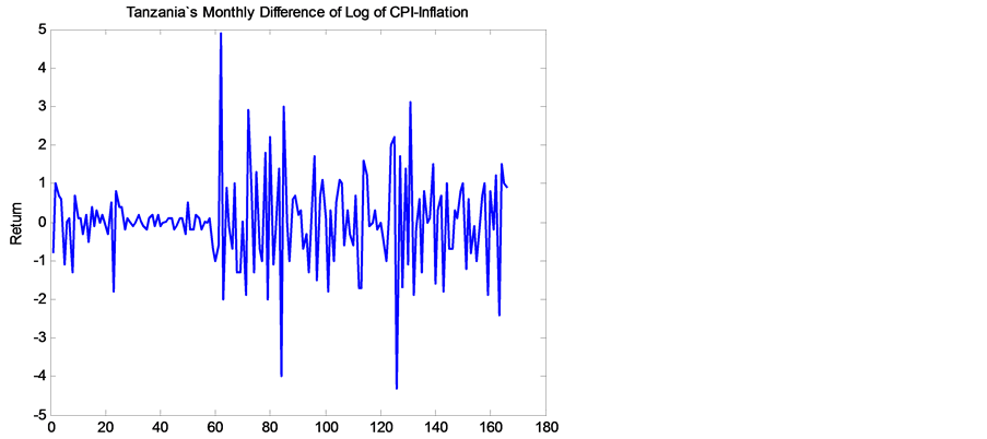
Figure 2. First difference of Log of CPI.
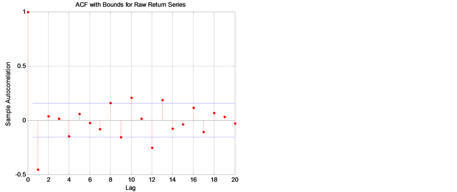
Figure 3. ACF with bounds for raw return series.
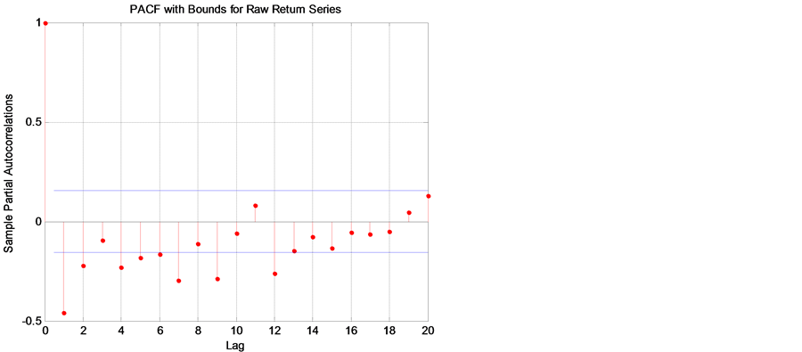
Figure 4. PACF with bounds for the raw returns series.
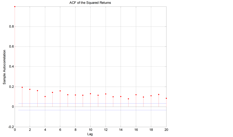
Figure 5. ACF of the squared returns.
Table 2. Ljung-Box-Pierce Q-test for autocorrelation (at 95% confidence).
Table 3. Ljung-Box-Pierce Q-test for squared returns (at 95% confidence).
Table 4. Engle ARCH test for heteroscedasticity (at 95% confidence).
From Table 2 it can be seen that there is no significant correlation in the raw returns at the 5% level of significance since H = 0. However, there is significant serial correlation in the squared returns in Table 3 when tested with the same inputs.
Table 4 is the Engle’s test for return series which shows that there is a significant correlation in the series, indicating presence of ARCH effects that is heteroscedasticity. Each of these tests extracts the sample mean from the actual inflation series.
4.2. Model Estimation and Evaluation
4.2.1. Model Selection
The strategy used in selecting the appropriate model from competing models is based
on the Akaike information criterion , the Bayesian information
criterion
, the Bayesian information
criterion
 and standard error
 and on the significance tests.
MATLAB software is used to perform trial and error evaluations to determine the
best fitting model. The idea is to have a parsimonious model that captures as much
variation in the data as possible. Usually the simple GARCH model captures most
of the variability in most stabilized series. Small lags for p and q are common
in applications. Typically GARCH , GARCH
 or GARCH
 models are adequate for modelling volatilities even over long sample periods [7]
.
models are adequate for modelling volatilities even over long sample periods [7]
.
From the derived models, using the method of maximum likelihood the estimated parameters
of GARCH model is summarized in the Table 5:


The standard errors are used to assess the accuracy of the estimates, the smaller
the better. The model fit statistics used to assess how well the model fit the data
are the AIC and BIC. The corresponding values are: AIC = 474.8 and BIC = 487.3 with
the log likelihood function of 233.4. The standard errors are quiet small suggesting
precise estimates. Based on 95% confidence level, the coefficients of the GARCH model are significantly different from zero and the estimated values satisfy the
stability condition, that is
model are significantly different from zero and the estimated values satisfy the
stability condition, that is .
.
Table 6 below summarizes fit statistics for the other GARCH models which were considered.
In conclusion, it can be established that, amongst all the identified models, the
GARCH proves the best fit model.
4.2.2. Diagnostic Checking of the GARCH(1,1) Model
One of the assumptions of GARCH models is that, for a good model, the residuals must follow a white noise process. Figure 6 inspects the relationship between the innovations (residuals) derived from the fitted model, the corresponding conditional standard deviations and the observed returns.
It can be observed that both innovations and returns exhibit volatility clustering. However if we plot the, standardized innovations (the innovations divided by their conditional standard deviation), they appear generally stable with little clustering as seen in Figure 7.
The time plot of the residuals given in Figure 7 is used to check whether the residuals are random. The normality check is also done by analyzing the histogram of residuals and normal probability plot. Figure 8 gives
Table 5. Parameter estimates for GARCH(1,1).
Table 6. Comparison of suggested GARCH models.
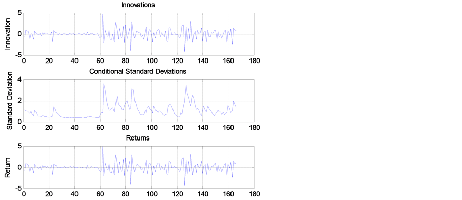
Figure 6. Plot for return, estimated volatility and innovations (residuals).
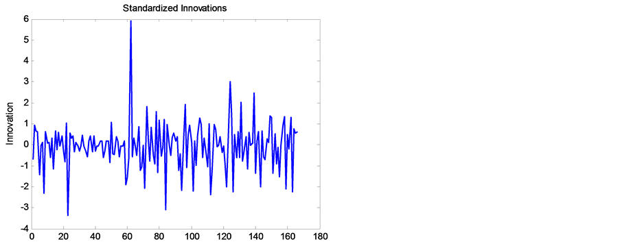
Figure 7. Time plot of residuals from GARCH(1,1).
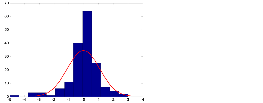
Figure 8. Histogram of residuals from GARCH (1, 1).
the histogram of the residuals from the GARCH(1,1) model. The histogram shows almost
a symmetric bellshaped distribution which is indicative of the residuals following
a normal distribution. The slight negative skewness is expected since the residuals
may also come from student’s
 distribution. The negative skewness tendency is also supported by negative large
residuals in Figure 7.
distribution. The negative skewness tendency is also supported by negative large
residuals in Figure 7.
Figure 9 gives the plot of the ACF of the squared
standardized innovations. The plot shows no correlation left.
Table 7 and Table 8 compare the results
of the
 and the ARCH test with the results of these same tests in the pre-estimation analysis
in Table 2 and Table 3
respectively. In the pre-estimation analysis, both the
and the ARCH test with the results of these same tests in the pre-estimation analysis
in Table 2 and Table 3
respectively. In the pre-estimation analysis, both the
 and the ARCH test indicated rejection (
 with
with
 value
value ) of their respective null hypothesis showing
significant evidence in support of GARCH effects. In the post estimation analysis
using standardized innovations based on the estimated model, these same tests indicate
acceptance (
) of their respective null hypothesis showing
significant evidence in support of GARCH effects. In the post estimation analysis
using standardized innovations based on the estimated model, these same tests indicate
acceptance ( with highly significant
 -values) of their respective null hypothesis
and confirm the explanatory power of GARCH
-values) of their respective null hypothesis
and confirm the explanatory power of GARCH . The tests showed that no
any ARCH effects left (no heteroscedasticity).
. The tests showed that no
any ARCH effects left (no heteroscedasticity).
4.3. Forecasting with the GARCH(1,1) Model
Table 7 shows the various measures of forecasting errors, namely the mean absolute error (MAE), the root mean squared error (RMSE), and Thiele’s U test for two models seemed to be adequately suitable to fit the data. The first two forecast error statistics depend on the scale of the dependent variable. These are used as relative measure to compare forecasts for the same series across different models. The smaller the error, the better the fore-
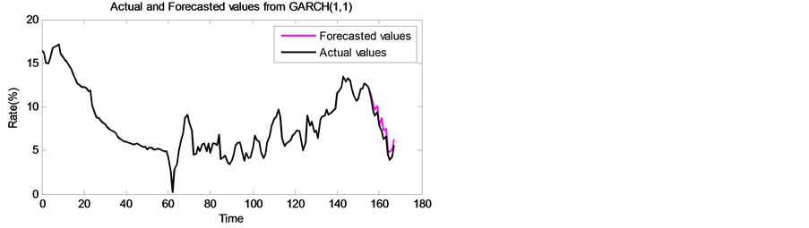
Figure 9. Time plot of inflation rate and one year forecasts by GARCH(1,1).
Table 7. Forecast Accuracy Test on the most likely suggested GARCH models.
Table 8. Inflation forecast by GARCH(1,1) model for period of January 2010 to December 2010.
casting ability of that model. The remaining two statistics are scale invariant. The Theil inequality coefficient always lies between zero and one, where zero indicates a perfect fit.
From Table 7, it can be seen that the accuracy
test favour GARCH model. Also the Thiele’s statistics is less than one (
 ) which indicates
that, the forecasts are fairly accurate. Table 8
below shows the forecast of Inflation by GARCH(1,1) for a period of one year from
January 2010 to December 2010.
) which indicates
that, the forecasts are fairly accurate. Table 8
below shows the forecast of Inflation by GARCH(1,1) for a period of one year from
January 2010 to December 2010.
The Figure 9 displays the actual inflation rate
and the predicted inflation rate by the GARCH model. The figure also displays how the forecasted values behave.
It can be observed from the Figure 9 that the forecasted inflation is closer to the actual inflation.
5. Discussion and Conclusion
In this paper, time series modelling was examined with a special application to modelling inflation data in Tanzania. In particular, the theory of univariate nonlinear time series analysis was explored and applied to the inflation data spanning from January 1997 to December 2010. The best fitting model was selected based on how well the model captures the stochastic variation in the data. Based on minimum Akaike Information Criteria (AIC) and Bayesian Information Criteria (BIC) values, it was observed that the best fit GARCH models were GARCH(1,1) and GARCH(1,2). However, after estimation of the parameters of selected models, a series of diagnostic and forecast accuracy test were performed and GARCH(1,1) model was found to be the best. Based on the selected model, twelve months inflation rates of Tanzania were forecasted in sample period (from January 2010 to December 2010). From the results, it is observed that the forecasted series are close to the actual data series.
References
- Ahiati, V.S. (2007) Discrete Time Series Analysis with ARMA Models. Revised Edition, Holden-Day, Oakland.
- Chatfield, C. (2000) Time Series Forecasting. Chapman and Hall, London.
- Webster, D. (2000) Webster’s New Universal Unabridged Dictionary. Barnes and Noble, New York.
- Hall, R. (1982) Inflation, Causes and Effects. Chicago University Press, Chicago.
- David, F.H. (2001) Modelling UK Inflation, 1875-1991. Journal of Applied Econometrics, 16, 255-275. http://dx.doi.org/10.1002/jae.615
- Engle, R. (1982) The Use of ARCH/GARCH Models in Applied Econometrics. Journal of Economic Perspectives, 15, 157-168. http://dx.doi.org/10.1257/jep.15.4.157
- Bollerslev, T. (1986) Generalized Autoregressive Conditional Heteroscedasticity. Journal of Econometrics, 31, 307- 327. http://dx.doi.org/10.1016/0304-4076(86)90063-1
- Amos, C. (2010) Time Series Modelling with Application to South African Inflation Data. Master’s Thesis, University of Kwazulu Natal, Kwazulu Natal.
- Tsay, R.S. (2002) Analysis of Financial Time Series. John Wiley & Sons, Hoboken. http://dx.doi.org/10.1002/0471264105
- Shephard, N. (1996) Statistical Aspects of ARCH and Stochastic Volatility Time Series in Econometrics, Finance and Other Fields. Chapman and Hall, London.
- Bollerslev, T., Chou, R.Y. and Kroner, K.F. (1992) ARCH Modeling in Finance: A Selective Review of the Theory and Empirical Evidence. Journal of Econometrics, 52, 5-59. http://dx.doi.org/10.1016/0304-4076(92)90064-X
- Ljung, G.M. and Box, G.E.P. (1978) On a Measure of Lack of Fit in Time Series Models. Biometrika, 65, 297-303. http://dx.doi.org/10.1093/biomet/65.2.297
NOTES

*Corresponding author.