Received 20 April 2015; accepted 1 June 2015; published 5 June 2015

ABSTRACT

The current study investigates the predator-prey problem with assumptions that interaction of predation has a little or no effect on prey population growth and the prey’s grow rate is time dependent. The prey is assumed to follow the Gompertz growth model and the respective predator growth function is constructed by solving ordinary differential equations. The results show that the predator population model is found to be a function of the well known exponential integral function. The solution is also given in Taylor’s series. Simulation study shows that the predator population size eventually converges either to a finite positive limit or zero or diverges to positive infinity. Under certain conditions, the predator population converges to the asymptotic limit of the prey model. More results are included in the paper.

Keywords:

Exponential Integral Function, Gompertz Model, Population Growth, Predator, Prey

1. Introduction

The predator-prey problem has been interesting to many researchers [1] -[7] . Modelling population growth of interacting species involves differential equations [1] [2] . The biological species interact in many and complex ways that may affect the population compositions over time, due to natural or artificial or management reasons.

Predation can increase, decrease, or have little effect on the strength, impact or importance of interspecific competition [3] . They indicate that there are cases in which predation has very little effect on competitive interactions.

It is discussed in [4] that the net effects of interspecific species interactions on individuals and populations vary in both sign (positive, zero, negative) and magnitude (strong to weak). Interaction outcomes are context- dependent when the sign and/or magnitude change as a function of the biotic or abiotic context.

The predator-prey problem with the assumptions of little or no effect of predation on the prey population growth is studied in [6] [7] . In this study, the prey populations are assumed to grow according to logistic, Von Bertalanffy and Richards models. The results show that the predation affects the predator population in such a way that its growth either converges to a finite positive limit or to zero or diverges to positive infinity.

There are several options to consider among the generalized growth models [8] . These include, for example, generalized logistic, particular case of logistic, logistic, Richards, Von Bertalanffy, Brody, Gompertz, generalized weibull, weibull, monomolecular, mitscherlich and more. Behavior of the growth models has been further studied in [8] - [10] .

The following sections are presented as follows: predator-prey models are presented in Section 2; Gompertz model in Section 3; solution for the Predator-prey equations in Section 4; simulation study in Section 5; analysis of phase diagram and equilibrium points in Section 6; and conclusions in Section 7.

2. Predator-Prey Models

The classical Lotka-Volterra predator-prey model is given by:

(1)

where, , and are positive constants. The parameter is intrinsic growth rate of the prey, b is rate of consumption of prey by predator, c is mortality rate of predator at absence of prey and d is reproduction rate of predator due to consumption of prey.

In the present work, we consider the case when the interaction of the prey and predator populations leads to a little or no effect on growth of the prey population, that is. We also assume the parameter is a function of time. Thus the assumptions of the classical predator-prey model are relaxed. The proposed predator-prey model is [6] :

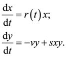(2)

where is population size or density of prey; is population size or density of predator communities in the system. Here we assume to be a relative growth rate function which is positive valued function of time. The parameter is reproduction rate of predator due to consumption of prey and is mortality rate of predator at absence of prey. Both are positive constants.

The prey Equation in (2) is the first order differential equation. The solutions of this first order differential equation are studied as growth models in [9] . This implies that a prey model can be selected from the large family of growth functions in [8] [9] . Given prey’s model, we can solve the differential equation of the respective predator population in (2).

The general approach for solving Equation (2) consists of the following steps:

1) Assume that the impact of predator on prey population growth is negligible,

2) Predator population declines in absence of prey,

3) Predator population grows with a rate proportional to a function of both and,

4) Assume that there is prior information about the prey population that follows a known growth function. Gompertz growth model in this case.

5) Solve for predator population growth.

3. Gompertz Model for Prey Population Growth

We assume that the growth of prey population follows Gompertz growth model and construct the corresponding predator growth function. The Gompertz model is given in [9] -[12] as follows:

(3)

where, is initial population size, is asymptotic growth of the population representing carrying capacity, and is absolute growth rate parameter of the prey. The respective relative growth rate is. The growth curve has a single point of inflection at time. Detailed discussion is found in [8] -[12] .

4. Solution of the Predator-Prey Equations

Here, we solve the ordinary differential equations in (2), then determine intersection points at which the prey and predator population attain same values, and finally three special cases of predator population are considered.

4.1. Derivation of the Model

The solution for the ordinary differential equation in (2) is derived assuming that prey follows the Gompertz model in (3). After substituting (3) in (2), the corresponding predator population growth function is derived to be:

(4)

Or equivalently,

(5)

where represents initial predator population size. The detailed derivations are given in Appendix 1.

Equation (4) is also equivalent to the following solution (6)―that can be expressed in terms of the well known exponential integral function Ei:

(6)

Note that the exponential integral function is a popular function that is often useful in many applications. We believe that this respective predator population growth function can be useful as well. In fact, Equation (6) can be expressed algebraically as the Ei function:

(7)

The predator models in Equations (4-7) appear to be new functions and they do not match with any one of the commonly known growth models.

4.2. Points of Intersection

Points of intersection are the point of time at which the prey and predator populations attain the same sizes.

Whenever it occurs, let the point of intersection be represented by, i.e. we must have in

Equations (3) and (4). In trying to solve these equations, we get the following expression expressed explicitly as:

where

Equation (7) can only be computed numerically.

4.3. Special Cases

To further understand the model in Equation (4), three special cases are identified which are dependent of birth and death parameters of predator population. The cases are considered here below.

Case I: In this case the function describing the population growth of predator in Equation (4) takes

the form. It is further observed that the predator

population converges to lower or upper asymptote depending on the initial value of the predator population. The initial population size can be larger or smaller than. Thus, the limiting value for the predator population is

.

It is interesting to note that both the prey and predator population sizes converge to the same asymptote provided that the parameter is assigned the value where. Also the predator population size converges to an asymptote above or below that of predator population size depending on or respectively.

Case II: In this case, the predator population decays from to zero as while the prey population grows from to.

Case III: In this case the predator population grows from and ultimately diverges to as while the prey population grows from to as expected or restricted.

The minimal point at which the predator growth curve turns or gets minimum value is found to be:. Then the values of prey and predator populations are and, respectively. This result is different, for example, for the case of logistic prey model [7] for which the minimum point occurs at and.

The cases can be generalized to a statement that ratio of deaths to births of predator growth is proportional to asymptote of prey growth. That is, where is a constant that can be related to an intervention factor applied on prey optimal size, or a factor that can be applied either to the predator’s birth para-

meter, or on the predator’s death parameter. Such intervention can hence be applied to the prey or predator parameters. The derivations provided in this paper correspond to the case that. For different from 1, the respective derivations can similar be made.

5. Simulation Study

The simulation study is carried out based on Equation (4). The study is designed by varying the model parameters: for prey population following Gompertz model and for predator population. The study design is as follows:

Prey model: Gompertz growth model

Prey model parameters:, ,.

Predator model parameters: is initial population size; birth rate, death rate.

Cases: Case I:, Case II:, Case III:

Case I: &; &; &; &; &

Case II: &; &; &; &

Case III: &; &; &; &

The results of the study are displayed in Figures 1-3.

Figure 1 displays plots for the Case I, where the ratio of death to birth of predator is equal to asymptotic size of prey A. In the simulation, the birth rate is varied from smaller to larger values. The result reveals that the predator population size decreases and eventually converges to a positive quantity at various rates. Note that for a particular value of the birth parameter , the population sizes of both prey and predator converge to same asymptotic value denoted by.

Figure 2 displays plots for the Case II, where the ratio of death to birth of predator is larger than A. For the simulation, we varied the rates with small magnitudes. The result shows that the predator population decreases over time and eventually converges to zero.

Figure 3 displays simulations for Case III, where the ratio death/birth of predator is less than A. Plots are made for various values of the rates. The result shows that the predator population declines for some time and then increases and eventually diverges to infinity.

We have shown by simulation study that the predator population either converges to a finite limit or converges to zero or diverges to infinity on the positive side depending on the parameter values under the assumption that prey follows Gompertz growth model. Moreover, for a particular value of birth parameter , the population sizes of both prey and predator converge to same asymptote. These findings are similar with those in [7] [8] .

6. Analysis of Phase Diagram and Equilibrium Points

The newly proposed predator-prey model (2) in its full form can be expressed, in case of Gompertz growth of prey population, as the system of equations and. The two equilibrium points of this system are found to be and since at both these points the necessary and sufficient conditions and are satisfied. Also the Jacobian matrix of the system of equations is. We now analyze the nature of the equilibrium points below and display the summary in Table 1.

Nature of the Equilibrium Point

The Jacobean matrix at this equilibrium point takes the form and the corresponding eigenvalues are and. Recall that all the parameters and are positive quantities and thus here arise the following two cases for while is always negative.

Condition I: In this case, both the eigenvalues and are negative and hence the equilibrium point is stable.

Condition II: In this case, the eigenvalues is positive while is negative and hence the equilibrium point is unstable.

Nature of the Equilibrium Point

The Jacobean matrix at this equilibrium point takes the form and the corresponding eigenvalues are and. The parameters and are positive and thus implies that is always negative but three cases for.

Condition I: In this case, is zero and hence the equilibrium point is stable.

Condition II: In this case, both the eigenvalues are negative and hence the equilibrium point is stable.

Condition III: In this case, only is positive. Hence the equilibrium point is unstable.

7. Conclusions

Some mathematical aspect of the well known predator-prey problem is studied by modifying the respective classical assumptions. We assume that the prey population growths naturally with no interaction effect due to predation and rate of growth is non-constant. Then, the predator-prey equations are solved considering prey grows as Gompertz model. The solution for the predator population is found to involve the exponential integral function and is equivalently expressed in terms of Taylor’s series.

The simulation studies and further analysis of the models reveal that the predator population grows in such a way that either converges to a finite limit or zero or diverges to positive infinity. There is a situation at which both prey and predator populations converge to the same limit irrespective of their initial population sizes. There is also a situation where the predator population attains a minimal point before it diverges to infinity. Moreover, two equilibrium points are identified which are stable only under some specific conditions.

References

Appendix 1

Derivation of Predator Population Model given Prey follows Gompertz Growth Model

Assume the prey population growth can be represented by the Gompertz function:

(i)

Then the predator equation can be solved as:

(ii)

Substituting (i) in (ii) gives

We now introduce a new variable for the purpose of evaluating the integral as

So as to get:

(iii)

To evaluate the integral, we now use Taylor’s series expansion of as:

or

Hence

(iv)

Using (iv) in (iii), we get:

(v)

To determine the integral constant we now impose the initial conditions and. That reduces (v) to be:

(vi)

To eliminate, subtract (vi) from (v) to get:

(vi)

But with,.

Thus, (vi) can be rearranged as:

(vii)

Thus is predator population size at. Using in (vii), we have

(viii)

The relationship (viii) is a phase path equation. It can be used to analyze phase path diagrams.

Appendix 2

Show the Solution with Exponential Integral Function and the Taylor’s Series of the Predator Population are Equivalent.

Exponential integral function, for small values of, is given by Maclaurin series as:

(i)

Here is called Euler’s constant. Using (i), the expressions for and can be obtained as follows:

(ii)

(iii)

On subtracting (iii) from (ii), we get

(iv)

But the expression can be simplified using (2) as

(v)

Hence, using (v) in (iv) we get

(vi)

Using (v) in (i), we get

Or equivalently

(vii)

Thus (vii) is the required predator equation expressed using exponential integral function. Since (vii) is derived from (i), it can be understood that both the solutions obtained using Taylor’s series expansion and Exponential integral function agree with each other.

Note that the indefinite integral together with the initial condition can be expressed as the semi-definite integral as. The lower limit is fixed.

NOTES

^*Corresponding author.

References

- Barnes, B. and Fulford, G.R. (2009) Mathematical Modelling with Case Studies: A Differential Equations Approach using Maple™ and MATLAB®. 2nd Edition, Chapman and Hall/CRC, London.
- Logan, J.D. (1987) Applied Mathematics―A Contemporary Approach. J. Wiley and Sons, Hoboken.
- Chase, J.M., Abrams, P.A., Grover, J.P., Diehl, S., Chesson, P., Holt, R.D., Richards, S.A., Nisbet, R.M. and Case, T.J. (2002) The Interaction between Predation and Competition: A Review and Synthesis. Ecology Letters, 5, 302-315. http://dx.doi.org/10.1046/j.1461-0248.2002.00315.x
- Chamberlain, S.A., Bronstein, J.L. and Rudgers, J.A. (2014) How Context Dependent are Species Interactions? Ecology Letters, 17, 881-890. http://dx.doi.org/10.1111/ele.12279
- Berlow, E.L. (1999) Strong Effects of Weak Interactions in Ecological Communities. Nature, 398, 330-334. http://dx.doi.org/10.1038/18672
- Gurevitch, J.J., Morrison, A. and Hedges, L.V. (2000) The Interaction between Competition and Predation: A Meta- Analysis of Field Experiments. The American Naturalist, 155, 435-453. http://dx.doi.org/10.1086/303337
- Dawed, M.Y., Koya, P.R. and Goshu, A.T. (2014) Mathematical Modelling of Population Growth: The Case of Logistic and Von Bertalanffy Models. Open Journal of Modelling and Simulation, 2, 113-126. http://dx.doi.org/10.4236/ojmsi.2014.24013
- Koya, P.R., Goshu, A.T. and Dawed, M.Y. (2014) Modelling Predator Population Assuming That the Prey Follows Richards Growth Model. European Journal of Academic Essays, 1, 42-51. http://euroessays.org/archieve/vol-1-issue-9
- Koya, P.R. and Goshu, A.T. (2013) Generalized Mathematical Model for Biological Growths. Open Journal of Modelling and Simulation, 1, 42-53. http://dx.doi.org/10.4236/ojmsi.2013.14008
- Koya, P.R. and Goshu, A.T. (2013) Solutions of Rate-State Equation Describing Biological Growths. American Journal of Mathematics and Statistics, 3, 305-311.
- Goshu, A.T. and Koya, P.R. (2013) Derivation of Inflection Points of Nonlinear Regression Curves―Implications to Statistics. American Journal of Theoretical and Applied Statistics, 2, 268-272.
- Winsor, C.P. (1932) The Gompertz Curve as a Growth Curve. Proceedings of the National Academy of Sciences of the United States of America, 18, 1-8. http://dx.doi.org/10.1073/pnas.18.1.1