Open Journal of Modelling and Simulation
Vol. 1 No. 4 (2013) , Article ID: 38842 , 12 pages DOI:10.4236/ojmsi.2013.14008
Generalized Mathematical Model for Biological Growths
School of Mathematical and Statistical Sciences, Hawassa University, Hawassa, Ethiopia
Email: drkpraocecc@yahoo.co.in, *ayele_taye@yahoo.com
Copyright © 2013 Purnachandra Rao Koya, Ayele Taye Goshu. This is an open access article distributed under the Creative Commons Attribution License, which permits unrestricted use, distribution, and reproduction in any medium, provided the original work is properly cited.
Received June 11, 2013; revised July 15, 2013; accepted August 1, 2013
Keywords: Growth Model; Koya-Goshu Function; Gompertz, Logistic; Richards; Weibull
ABSTRACT
In this paper, we present a generalization of the commonly used growth models. We introduce Koya-Goshu biological growth model, as a more general solution of the rate-state ordinary differential equation. It is shown that the commonly used growth models such as Brody, Von Bertalanffy, Richards, Weibull, Monomolecular, Mitscherlich, Gompertz, Logistic, and generalized Logistic functions are its special cases. We have constructed growth and relative growth functions as solutions of the rate-state equation. The generalized growth function is the most flexible so that it can be useful in model selection problems. It is also capable of generating new useful models that have never been used so far. The function incorporates two parameters with one influencing growth pattern and the other influencing asymptotic behaviors. The relationships among these growth models are studied in details and provided in a flow chart.
1. Introduction
Measuring biological growth has been important in many fields. Many researchers have contributed in developing relevant models: [1] for Brody function; [2] for Von Bertalanffy function; [3,4] for Richards function; [5] for Gompertz function; [6-8] for Logistic function; [6,9-11] for Generalized Logistic; [12,13] for Weibull function; [1,14] for Monomolecular function.
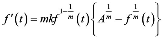
The mathematical representation of the relative growth is described by the ordinary differential equation (ODE) or rate-state equation
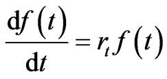 (1)
(1)
Here  is representing growth function and
  is relative rate function at time
 . This ordinary differential equation has many solutions among which some are studied in this paper. The growth models have been widely used in many biological growth problems including: in animal sciences [1,5,7,8,15,16] and in forestry [17,18]. Simulation studies by [19] indicate that such growth functions are so flexible to wrongly fit to given data set and recommends more care while selecting the models.
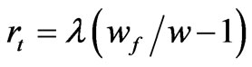
A number of attempts have been made to generalize the growth models. For example, [17] modified the ODE
(1) by including one parameter  as:
as:
 from which some growth models are derived. Moreover, they have shown that the model has upper limit but no inflection point when
 ; and has both upper limit and inflection point for
 .
.
[18] defined 9-parameters model as: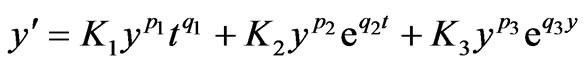 . The first two terms include all commonly known growth functions except Weibull, and so they included to the third term to account for it.
The generalized logistic function has been studied by some researchers [6,9-11]. Eberhardt and Breiwick [9] applied the models to growth of birds and mammals populations.
In the current paper, we provide a new single generalized growth model as solution of the ODE (1) consisting of eight parameters. It can also serve for model selection purposes. We also study the mathematical relationships among the models presented herein. Inflection points of the models are discussed.
2. Koya-Goshu Growth Function as a Generalization of Growth Functions
In this section we define a new generalized growth function, named as Koya-Goshu growth function and show how it accommodates the commonly known growth models such as: Logistic, Generalized Logistic, Gompertz, Brody, Monomolecular, Mitscherlich, Von Bertalanffy, Richards, Generalized Weibull and Weibull functions.
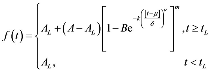
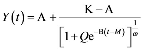
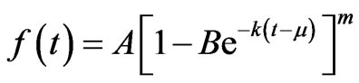
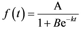
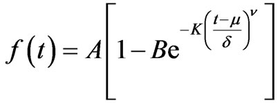
The new generalized growth function, Koya-Goshu growth function, is defined as
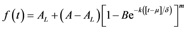 (2)
(2)
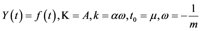
Here the parameters are defined as follows:
 is derived from
 , A is upper asymptote of
 : Lower asymptote of
 Growth rate parameter
 Time shift, a constant
 Time scale, a constant
 Shape parameters of the growth function,
2.1. Description of Koya-Goshu Growth Model
The Koya-Goshu growth model is 8-parameter  function. The model is a more general solution of the ODE (1). Note that
  and equal at time
  Regarding the quantity
 ,
,  as
as ;
;  as
as ;
;  as
as . The quantity
  can assume any value in the open interval
  for Richards, and in (0, 1) for both Von Bertalanffy and Brody. For both Logistic and Gompertz,
  can take any positive real number. For Weibull,
  while for generalized Weibull case,
 .
.
When time  is non-negative, the Koya-Goshu function is well defined for modeling growths. The function represents sigmoid curve for m < 0 and
  any positive odd integer. However, if m > 0 or (m < 0 and
  is any real number other than positive odd integer), the function is well defined growth model for time
  where
where
 . This implies that the function misses lower asymptote in some cases. To account for the asymptote, modification can be made by taking
  for
for  or can be written as:
Thus, the Koya-Goshu function in (2) can be generally expressed as:
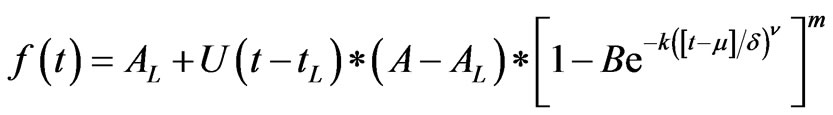 (3)
(3)
Here * is used to denote multiplication. Also here
 is a unit step function, where
 if
if  or
or
if

 is a lower bound for the time. Note that
  with
with  defined by the limit of
  as time t goes to
 . It serves as a lower asymptote of
 .
.
Note that the Koya-Goshu function is defined at all points  in
in  -plane. All the commonly known growth curves lay along the line
  or
or  only. The function extends the inclusion of other points in the plane than these points. This means that it is so flexible that one can select any other curves than the commonly used ones.
We show that the Koya-Goshu model accommodates all commonly known growth functions. We have given detailed analysis of the growth models and how they are related to each other. The Richards function is a general form of Brody, Von Bertalanffy, Classical Logistic and Gompertz. Brody is same as Monomolecular and Mitscherlich functions. Brody is a special case of Weibull function. All the relations are illustrated by flow chart in Figure 1. Detailed derivations of the function  and relative growth rate
  are given in Appendix A.
Some selected plots are illustrated in Figures 2-5.
2.2. Properties of the Koya-Goshu Function
The function represents both increasing and decaying growths (see Figure 2(a), 3(a), 4(a), 5(a)). It is increasing for  and decaying for
 . This means that increasing or decaying of the growth is influenced by sign (positive or negative) of
 , irrespective of the values of m.
The function represents increasing growths with upper asymptote but no lower asymptote:
1) For all positive combination values of both  and
and  (see Figures 2(a), 3(a))
2) For all small negative values of  and large positive values of
  (see Figure 4(a)).
The function represents increasing growths with both upper and lower asymptotes:
1) For all negative values of m and any (small or large)
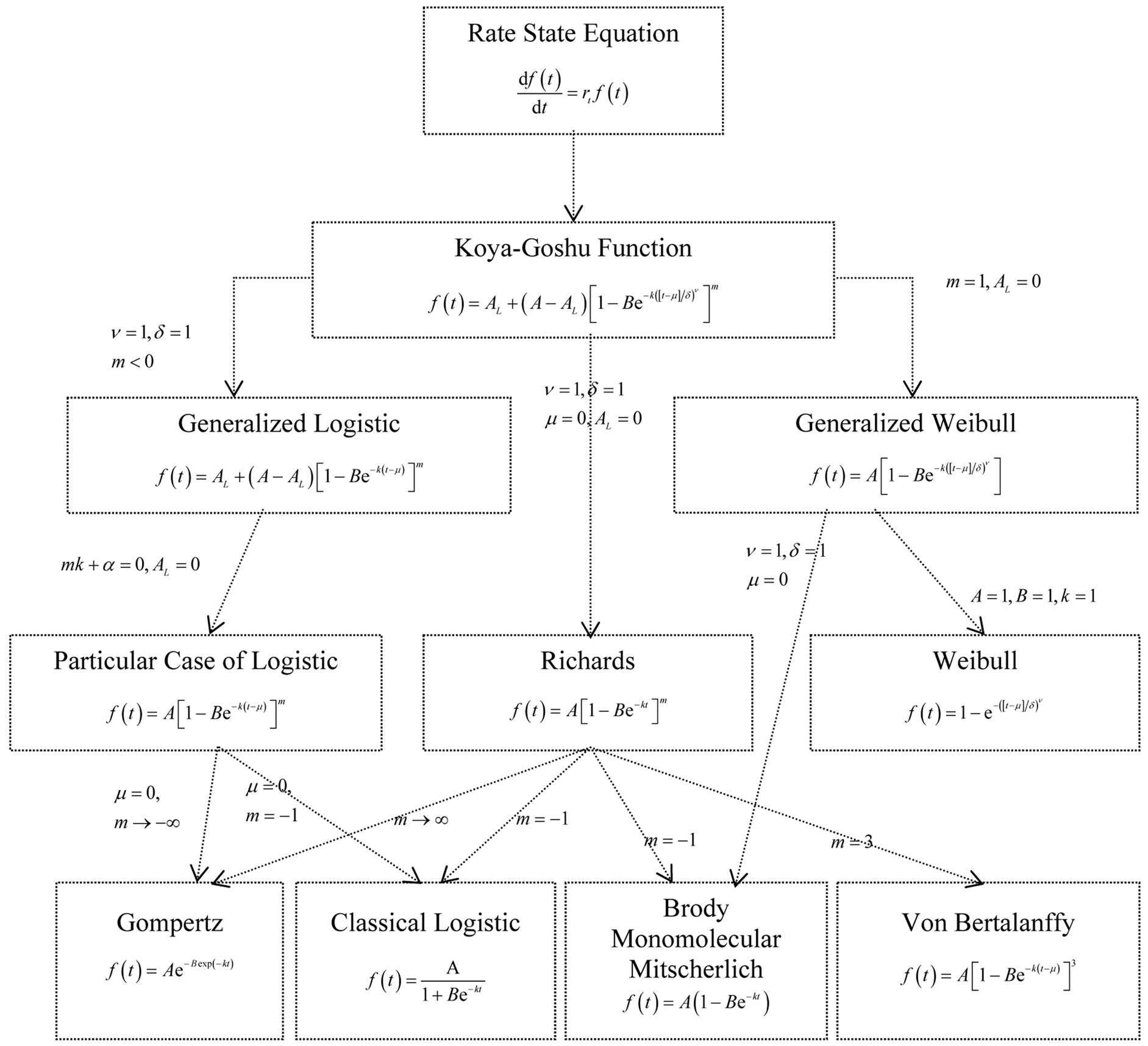
Figure 1. Flow chart illustrating the relationships among the generalized and specialized growth functions.
 (a)
(a) (b)
(b)
Figure 2. Plots of (a) growth functions and (b) rate functions with .
.
 (a)
(a) (b)
(b)
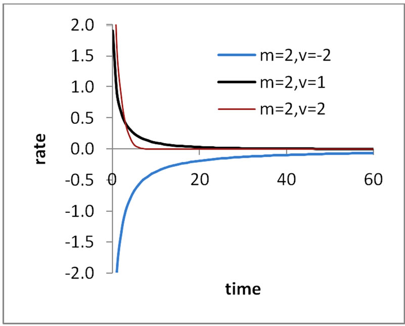
Figure 3. Plots of (a) growth functions and (b) rate functions with .
.
 (a)
(a)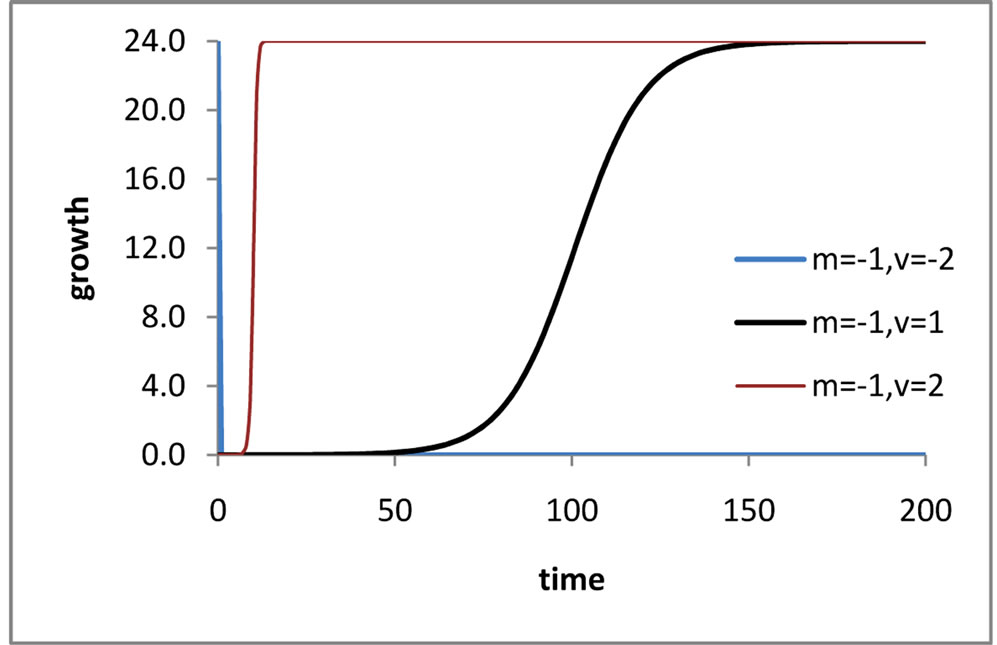 (b)
(b)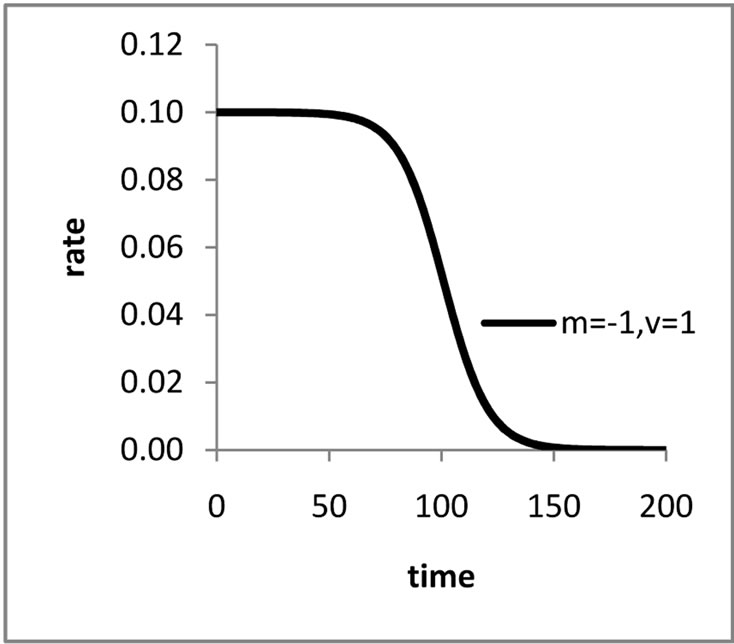 (c)
(c)
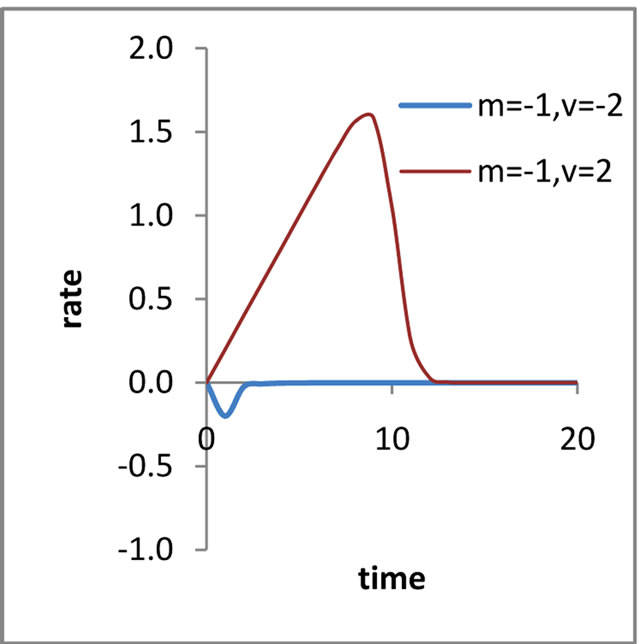
Figure 4. Plots of (a) growth functions and (b) (c) rate functions with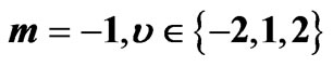 .
.
positive values of  (see Figure 5(a))
2) For all small negative values of  and small positive values of
  (see Figure 4(a)).
The occurrence of either lower and upper asymptotes or only upper asymptotes is influenced by only  but not
 . Generally, the parameter
  influences growth behavior, while the parameter
  influences asymptotic behavior of the function.
 (a)
(a) (b)
(b)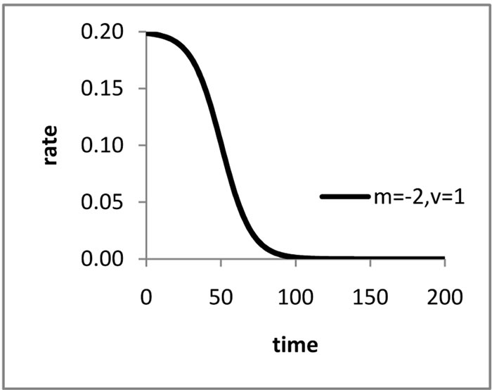 (c)
(c) (d)
(d)
Figure 5. Plots of (a) (b) growth functions and (c) (d) rate functions with .
.
2.3. Inflection Point of Koya-Goshu Function
We now introduce the definition of inflection points of a curve, and describe the procedure to find inflection points for the growth functions we discuss in this paper. Suppose that the function  is continuous on an open interval containing the point
 . Then the point
  is called an inflection point of
  provided that
  on one side of
  and
and  on the other side. At the inflexion point
  itself either
  or
or  does not exist [20].
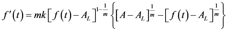
 (4)
(4)
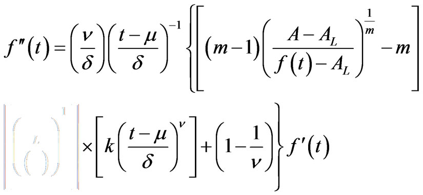 (5)
(5)
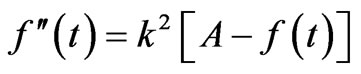
Here, we observe that
 (6)
(6)
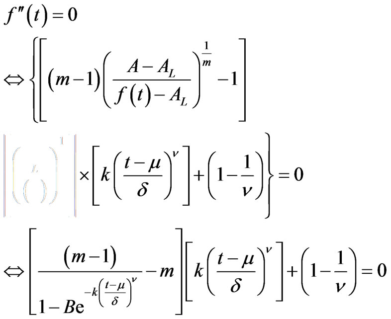
Clearly, point of inflection exists in Koya-Goshu function provided the relation (5) is satisfied, since  at that point and also
  and
and  are satisfied on the increasing and decreasing sides of that point.
Here it can be observed that the inflection points of Koya-Goshu function, when the parameters are fixed as 1) , and 2)
  perfectly matches with the cases of Generalized logistic functions and Generalized Weibull models, respectively.
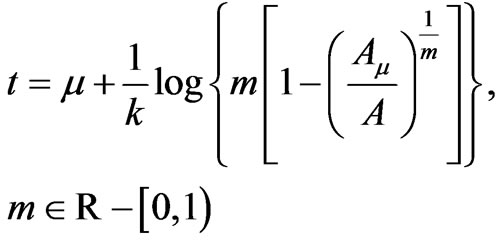
For the other cases when , the inflection point for the Koya-Goshu function can be obtained by approximations. For example, using Taylor series expansion up to first order term, the time of inflection is approximated as:
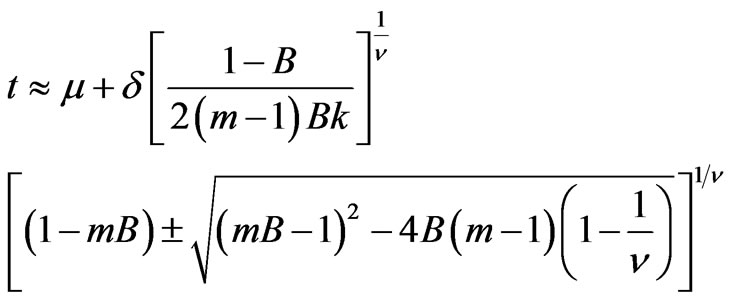 (7)
(7)
3. Biological Growth Models and the Parametric Relationships
In this section we studied the parametric relationships among all the biological growth models considered in this paper viz., Koya-Goshu biological growth model, Generalized Logistic, Particular case of Generalized Logistic, Richards, Von Bertalanffy, Brody, Logistic, Gompertz, Generalized Weibull, Weibull Monomolecular, and Mitscherlich functions. The relationships identified have been exhibited through a flowchart.
3.1. Generalized Logistic Function
The Generalized Logistic function as given in [21] is expressed in its original notations as
 which we now re-express it with same notations used in this paper as
 (8)
(8)
by replacing in the equation 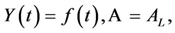
 and
and
 .
.
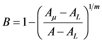
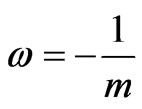
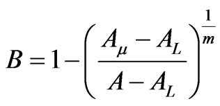
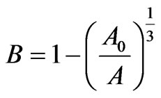
The Generalized Logistic function (7) is hereby a special case of Koya-Goshu function with  and
and . The parameter B takes the form
 . The expression for the relative growth rate function can be computed as
  . Similarly, the expressions for
  and
and  are, respectively, given by
 and
and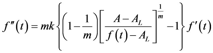 .
.
The single point of inflection occurs when the organism reaches the growth 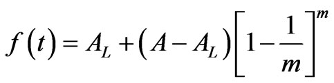
 at time
where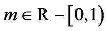 . For
. For , inflexion point does not exist.
3.2. Particular Case of the Generalized Logistic Function
A function called Particular case of the Generalized Logistic function is defined [21] as
 which we now re-express it with same notations used in this paper as
 (9)
(9)
by replacing in the equation
 and
and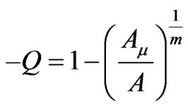 . Note that Equation (8) is a special case of Equation (7) for Generalized Logistic function with
 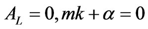 In this case, the parameter
takes the form as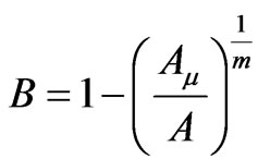 . The expression for the relative growth rate function
  can be computed as
 . Similarly, the expressions for
  and
and  are respectively given by
 and
and . The single point of inflection occurs when the organism reaches the growth
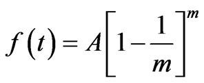
 at time
For , inflexion point does not exist.
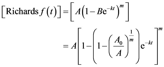
3.3. Richards Function
The Richards function is defined as in the usual notations (Richards, 1959) as
 (10)
(10)
Here . The Richards function can be directly derived from the ODE or rate-state Equation (1)
with relative rate function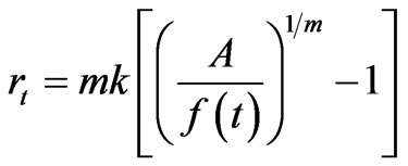 . The Richards function becomes special case of Koya-Goshu growth model with
 . Here the parameter m can assume any non-zero real number. The expressions for
  and
and  are given by respectively
 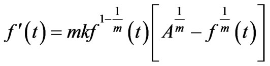 and
and 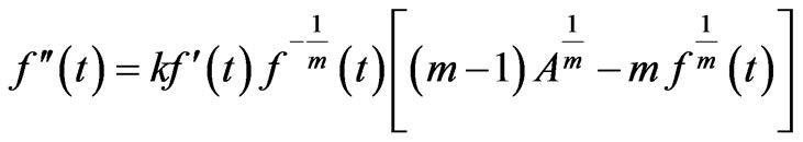 The single point of inflection occurs when the growth reaches
  of its final growth, i.e.
 at time
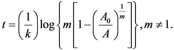
3.4. Von Bertalanffy Function
Von Bertalanffy is defined (Bertalanffy, 1957) as
 (11)
(11)
It is a special case of Richards function (5) with  and a special case of Koya-Goshu growth model with
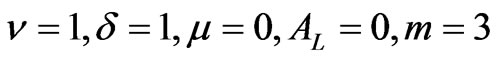 . Here
 . It can also be derived from ODE (1) with relative rate function
 . For Von Bertalanffy function
  and
and  are respectively given by
 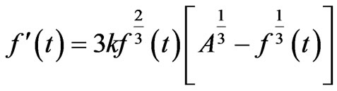 and
and 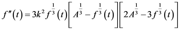 . Here the single point of inflection occurs when the growth reaches
 of its final growth, i.e.

 at time
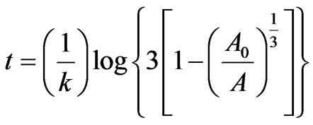 .
.
3.5. Brody Function
Brody is defined (Brody, 1945) as:
 (12)
(12)
It is a special case of Richards function (9) with  and a special case of Koya-Goshu growth model with.
 . It can also be derived from ODE (1) with rate function
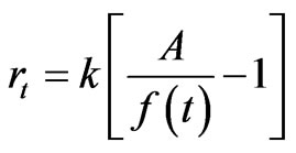 . Here
  and
and  are respectively given by
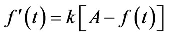 and
and
 . Brody growth function does not possess a point of inflexion since
  is not satisfied for any value of
 .
.
3.6. Logistic Function
The classical Logistic function (Nelder, 1961) is defined as:
 (13)
(13)
Here . The Logistic function is a special case of 1) Richards function (9) with
2) Particular case of logistic function (8) with 
3) Generalized logistic function (7) with 
4) Koya-Goshu function (2) with  .
.
The Logistic function can be derived from the ODE (1) with rate function
 . Here,
  and
and  are respectively given by
 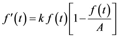 and
and 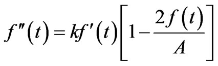 . The single point of inflection occurs when the growth reaches half of its final growth
  at time
 .
.
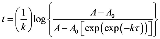
3.7. Gompertz Function
The Gompertz function (Winsor, 1932) is defined as
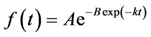 (14)
(14)
where .
.
It is shown to be a special case of 1) Richards function (9) with  2) Particular case of logistic function (8) with
  3) Generalized logistic function (7) with
 ,
,  4) Koya-Goshu function (2) with
 . The Gompertz function can be derived from the ODE (1) with rate function
 . Here,
 ,
,
 and the single point of inflection occurs when the growth reaches
  of its final growth, i.e.,
  at time
 .
.
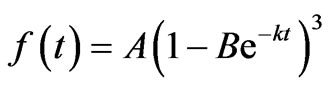
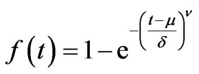
3.8. Generalized Weibull Function
The Weibull function is generalized and named here by Generalized Weibull function as
 (15)
(15)
where . The generalized Weibull is a special case of Koya-Goshu growth function (2) with
 . Generalized Weibull functions can be derived from the ODE (1) with rate function
 . For Generalized Weibull,
  and
and  are respectively given by
 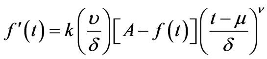 and
and  . The single point of inflection occurs when the organism reaches the growth
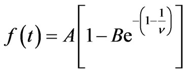
 at time
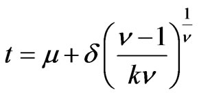 .
.
3.9. Weibull Function
The Weibull growth model (Rawlings et al., 1998) is given as
 (16)
(16)
The Weibull function can be derived from the ODE (1)
with rate function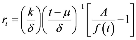 .
.
Weibull a special case of Generalized Weibull (13) function with  and that of Koya-Goshu growth function (2) with
 . For Weibull,
  and
and  are respectively given by
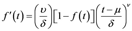 and
and  . For Weibull, the single point of inflection occurs when the organism reaches the growth
 at time
 . This fact can be verified by directly substituting
  in the inflection point of Generalized Weibull.
3.10. Monomolecular and Mitscherlich Functions
Here we show that Brody, Monomolecular and Mitscherlich growth functions are the same, except that the names and notations used are different. Hence, all these three functions exhibit the same properties and behaviors and also they represent the same growth patterns.
Monomolecular growth function is defined (France et al., 1996), in its original notations, as
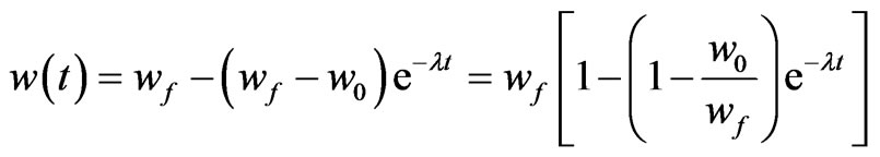
where  is the growth function at time
 ,
,  is the final (mature) value,
  at
at  is the initial value and
  is rate of growth. This function can be expressed as Brody function (7) with notations

as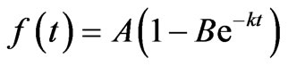 . Monomolecular growth function can be derived from the ODE (1) with rate function
 or
or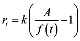 .
.
Thus, Monomolecular growth function, just similar to Brody growth function, does not possess a point of inflexion since  is not satisfied for any value of
 .
.
Mitscherlich growth function [22] is defined, in its original notations, as 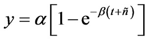 where
where  is the growth function at time
 ,
, ![]() is the final (mature) growth,
is the final (mature) growth,  is a constant and
  is rate of growth. The Mitscherlich function can be expressed with notations
 as Brody function
  given by (7). It can be derived from the ODE (1) with rate function
 or
or .
.
Not that the integral constant becomes 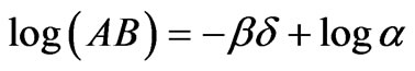 . Thus, Mitscherlich growth function, just similar to Brody growth function, does not possess a point of inflexion since
  is not satisfied for any value of
 .
.
4. Other Relationships
Here we derive explicitly and present few more relationships, other than those mentioned in Section 3, among the growth models considered in this paper.
4.1. Relation between Richards and Logistic Functions
Let us now see how Richards and Logistic functions are related. Using the Richards function (9), we can derive Logistic (12) as follows:
 (17)
(17)
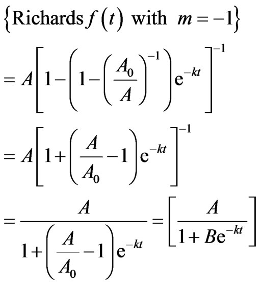 (18)
(18)
where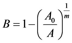 . Hence, Richards growth function with
  leads to the Logistic function.
4.2. Relation between Richards and Gompertz Functions
We now show how Gompertz is related to Richards function, i.e., the relative growth rate function of Richards as ![]() leads to that of Gompertz, which is now shown. Note that the relative growth rate functions of Gompertz and Richards are given respectively by
leads to that of Gompertz, which is now shown. Note that the relative growth rate functions of Gompertz and Richards are given respectively by
 and
and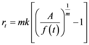 .
.
By applying the limit as  on Richards
 , we get the following:
 (19)
(19)
Here the last expression is obtained by a simple algebraic rearrangement of the expression. In this expression evaluation of limit leads to  and to avoid that we applying L-Hospital rule to get
 (20)
(20)
Thus, the limiting value of the Richards relative rate growth function as  reduces to the Gompertz relative rate growth function, and hence these two functions are related.
4.3. Relation between Particular Case of Generalized Logistic and Gompertz
We now show how Gompertz is related to the particular case of generalized Logistic function, i.e., the relative growth rate function of the particular case of generalized Logistic as  leads to that of Gompertz, which is now shown. Note that the relative growth rate functions of Gompertz and the particular case of generalized Logistic are given respectively by
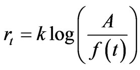 , and
, and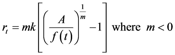 .
.
By applying the limit as  on
on  of the particular case of generalized Logistic function, we get the following:
 (21)
(21)
Here the last expression is obtained by a simple algebraic rearrangement after the inverse functions viz, logarithmic and exponential operations are used. In this expression evaluation of limit leads to  and to avoid that we apply L-Hospital rule to get
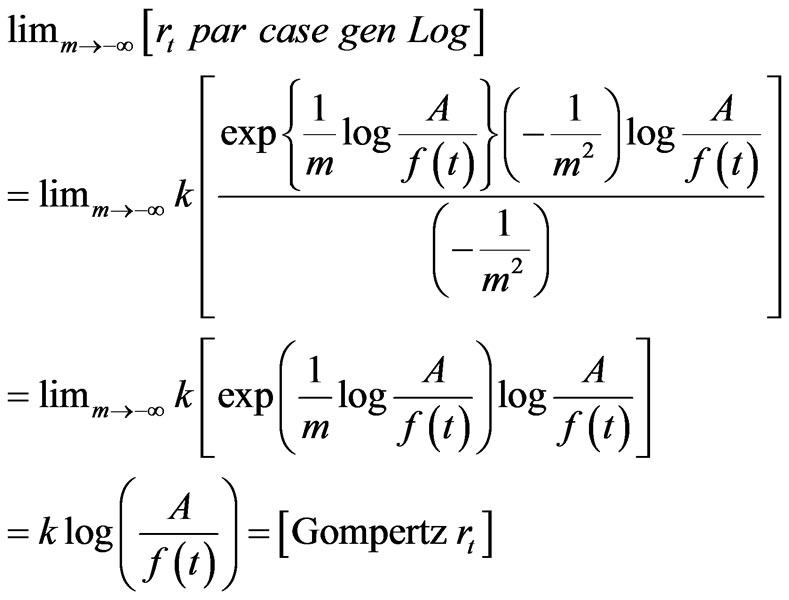 (22)
(22)
Thus, the relative rate growth function the particular case of generalized logistic function as  reduces to the Gompertz relative rate growth function, and hence these two functions are related.
4.4. Relation between Brody and Gompertz Functions
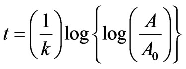
We have shown in the flow chart the relationships among the growth functions by setting the parameters suitably. However, Gompertz and Brody functions can be related through a transformation of time coordinate and that goes as follows:
Let the time variables of Brody and Gompertz are represented by  and
and  respectively. Now consider the Brody function as
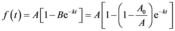 (23)
(23)
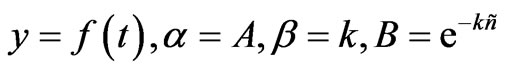
and the Gompertz function as
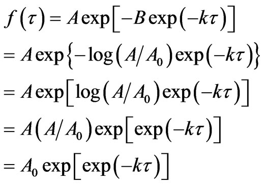 (24)
(24)
Now on equating the  and
and  from (23) and (24), we get
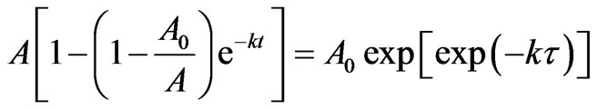 (25)
(25)
and this can be expressed as
 (26)
(26)
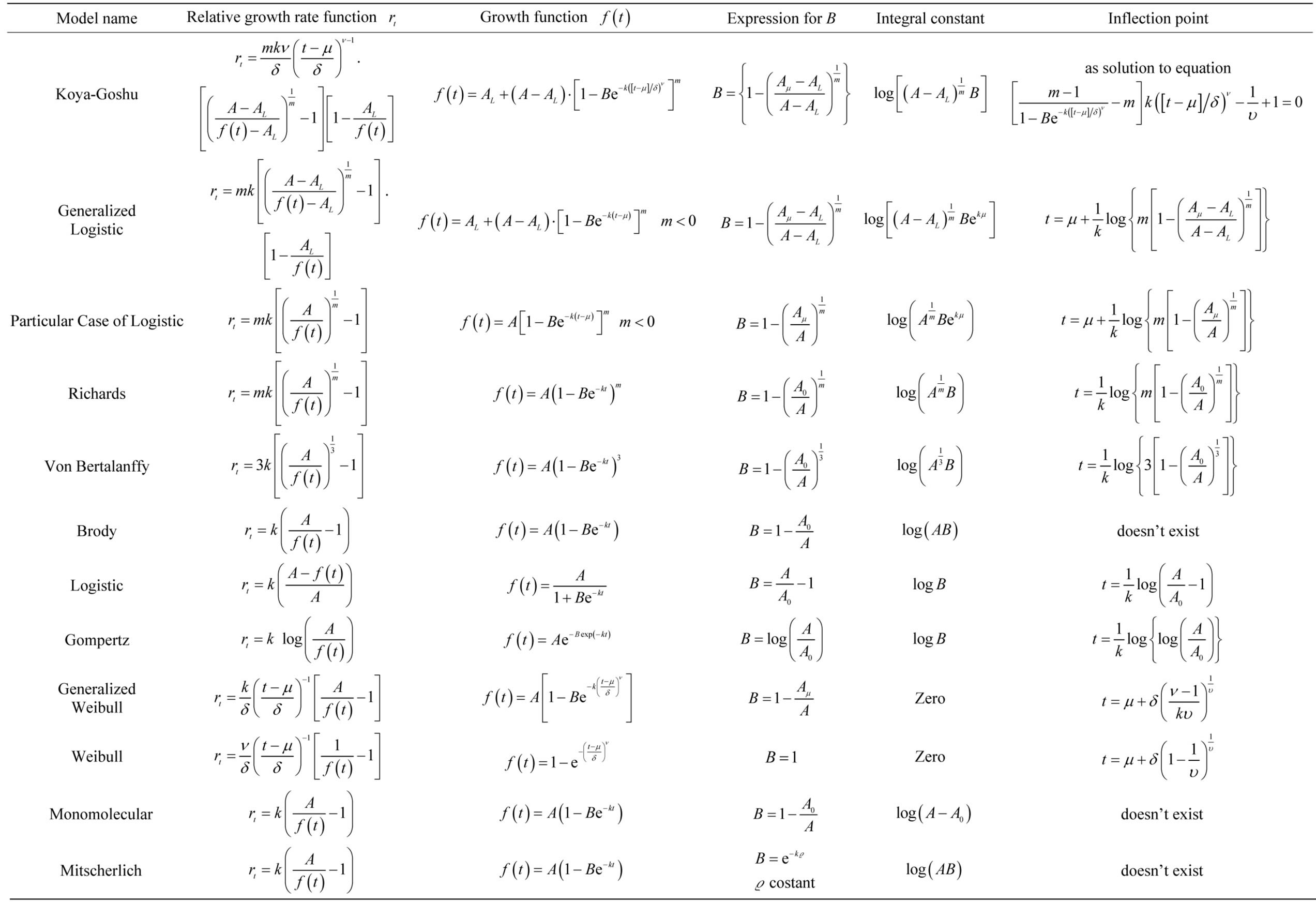
Table 1. List of growth functions and their respective rate functions, expressions for b, integral constants and inflection points.
which is the coordinate transformation equation between the time variables of Brody and Gompertz functions.
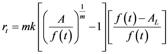
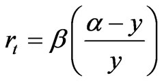
5. Illustration for How Relative Growth Rate Function Behaves—Richards Case
The relative growth rate function  is significantly different for the models at early ages and converges to zero for the later ages. The relative growth rate
  is an increasing function of
  while it is a decreasing with time t. However,
  grows with
  in the early ages allowing the parameter m to play a significant role. Subsequently,
  dies at later ages irrespective of
 . We consider Richards function as example to illustrate this.
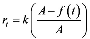
Consider the Richards relative growth rate function :
:
 (27)
(27)
is a function of parameter  and time
 , and limit gives:
 (28)
(28)
Equation (28)  is increases with
  at early times.
Also, on taking the limit of  in (27) as
 , we get

showing that  vanishes at time of growth maturity for all
 .
.
6. Conclusion
This paper introduces a new generalized mathematical model for biological and other growths, named as KoyaGoshu growth model. It is a generalization of the commonly used growth functions such as: Brody, Von Bertalanffy, Richards, Weibull, Monomolecular, Mitscherlich, Gompertz, Logistic and generalized Logistic functions. Koya-Goshu model is constructed as a solution of ordinary differential or rate-state equation. The function incorporates two parameters where one influences growth pattern and the other influences asymptotic behavior. The model is so flexible that it can be useful in model selections. Moreover, it generates new and useful growth functions. All of the growth models considered under the study are related to each other as illustrated in the flaw chart. As further studies, we will take up applications of this model for data fitting and prediction.
REFERENCES
- S. Brody, “Bioenergetics and Growth,” Reinhold Publishing Corporation, New York, 1945.
- L. von Bertalanffy, “Quantitative Laws in Metabolism and Growth,” The Quarterly Review of Biology, Vol. 3, No. 2, 1957, p. 218.
- F. J. Richards, “A Flexible Growth Function for Empirical Use,” Journal of Experimental Botany, Vol. 10, 1959, pp. 290-300. http://dx.doi.org/10.1093/jxb/10.2.290
- J. France and J. H. M. Thornley, “Mathematical Models in Agriculture,” Butterworths, London, 1984, p. 335.
- C. P. Winsor, “The Gompertz Curve as a Growth Curve,” Proceedings of National Academy of Science, Vol. 18, No. 1, 1932, pp. 1-8. http://dx.doi.org/10.1073/pnas.18.1.1
- J. A. Nelder, “The Fitting of a Generalization of the Logistic Curve,” Biometrics, Vol. 17, No.7, 1961, pp. 89- 110. http://dx.doi.org/10.2307/2527498
- J. E. Brown, H. A. Fitzhugh Jr. and T. C. Cartwright, “A Comparison of Nonlinear Models for Describing WeightAge Relationship in Cattle,” Journal of Animal Science, Vol. 42, No. 4, 1976, pp. 810-818.
- T. B. Robertson, “On the Normal Rate of Growth of an Individual and Its Biochemical Significance,” Archiv für Entwicklungsmechanik der Organismen, Vol. 25, No. 4, 1906, pp. 581-614. http://dx.doi.org/10.1007/BF02163864
- L. L. Eberhardt and J. M. Breiwick, “Models for Population Growth Curves,” ISRN Ecology, Vol. 2012, 2012, Article ID: 815016. http://dx.doi.org/10.5402/2012/815016
- D. Fekedulegn, M. P. Mac Siurtain and J. J. Colbert, “Parameter Estimation of Nonlinear Growth Models in Forestry,” Silva Fennica, Vol. 33 No. 4, 1999, pp. 327-336.
- F. J. Ayala, M. E. Gilpin and J. G. Ehrenfeld, “Competition between Species: Theoretical Models and Experimental Tests,” Theoretical Population Biology, Vol. 4, No. 3, 1973, pp. 331-356. http://dx.doi.org/10.1016/0040-5809(73)90014-2
- J. O. Rawlings and W. W. Cure, “The Weibull Function as a Dose Response Model for Air Pollution Effects on Crop Yields,” Crop Science, Vol. 25, 1985, pp. 807-814. http://dx.doi.org/10.2135/cropsci1985.0011183X002500050020x
- J. O. Rawlings, S. G. Pantula and D. A. Dickey, “Applied Regression Analysis: A Research Tool,” Springer, New York, 1998.
- W. J. Spillman and E. Lang, “The Law of Diminishing Increment,” World, Yonkers, 1924.
- J. France, J. Dijkstra and M. S. MDhanoa, “Growth Functions and Their Application in Animal Science,” Annales De Zootechnie, Vol. 45, Suppl. 1, 1996, pp. 165-174. http://dx.doi.org/10.1051/animres:19960637
- I. E. Ersoy, M. Mendeş and S. Keskin, “Estimation of Parameters of Linear and Nonlinear Growth Curve Models at Early Growth Stage in California Turkeys,” Archiv für Geflügelkunde, Vol. 71, No. 4, 2007, pp.175-180.
- Y. C. Lei and S. Y. Zhang, “Features and Partial Derivatives of Bertalanffy-Richards Growth Model in Forestry,” Nonlinear Analysis: Modelling and Control, Vol. 9, No. 1, 2004, pp. 65-73.
- B. Zeide, “Analysis of Growth Equations,” Forest Science, Vol. 39, No. 3, 1993, pp. 594-616.
- A. T. Goshu, “Simulation Study of the Commonly Used Mathematical Growth Models,” Journal of the Ethiopian Statistical Association, Vol. 17, 2008, pp. 44-53.
- C. H. Edwards Jr. and D. E. Penney, “Calculus with Analytic Geometry,” Printice Hall International, New Jersey, 1994.
- Generalised logistic function http://en.wikipedia.org/w/index.php?oldid=472125857
- R. A. Mombiela and L. A. Nelson, “Relationships among Some Biological and Empirical Fertilizer Response Models and Use of the Power Family of Transformations to Identify an Appropriate Model,” Agronomy Journal, Vol. 73, No. 2, 1981 pp. 353-356. http://dx.doi.org/10.2134/agronj1981.00021962007300020025x
NOTES
*Corresponding author.