Advances in Aerospace Science and Technology
Vol.04 No.02(2019), Article ID:93335,13 pages
10.4236/aast.2019.42003
Predictive Control of Quad-Rotor Delivering Unknown Time-Varying Payloads Based upon Extended State Observer
Yuan Wang
Key Laboratory of Fundamental Science for National Defense-Advanced Design Technology of Flight Vehicle, Nanjing University of Aeronautics and Astronautics, Nanjing, China

Copyright © 2019 by author(s) and Scientific Research Publishing Inc.
This work is licensed under the Creative Commons Attribution International License (CC BY 4.0).
http://creativecommons.org/licenses/by/4.0/


Received: May 30, 2019; Accepted: June 25, 2019; Published: June 28, 2019
ABSTRACT
In this paper, robust control problem is addressed for quad-rotor delivering unknown time-varying payloads. Firstly, the model of a quad-rotor carrying payloads is built. Dynamics of the payloads are treated as disturbances and added into the model of the quad-rotor. Secondly, to enhance system robustness, the extended state observer (ESO) is applied to estimate the disturbances from the payloads for feedback compensation. Then a type of predictive controller targeting multiple-input-multiple-output (MIMO) system is developed to degrade the influences caused by sudden changes from loading/dropping of the payloads. Finally, by making comparison with the conventional cascade proportional-integral-derivative (CPID) and the sliding mode control (SMC) approaches, superiority of the scheme developed is validated. The simulation results indicate that the CPID method shows poor performance on attitude stabilization and the SMC shows input chattering phenomenon even it can achieve satisfied control performances.
Keywords:
Quad-Rotor, Payloads Delivery, Attitude Control, Disturbance Estimation, Feedback Compensation, Predictive Control

1. Introduction
During the past decades, quad-rotor has been applied in many fields such as succor, inspection, surveillance and aerial cinematography. To meet task requirements with high reliability, many effective approaches were developed, such as proportional-integral-derivative (PID) [1] , linear quadratic regulator (LQR) [2] , model reference adaptive control (MRAC) [3] , feedback linearization (FL) [4] , sliding model control (SMC) [5] and back-stepping (BS) [6] and so forth. In recent years, package delivery has become an important application for quad-rotors, such as Amazon’s and DHL’s drone package delivery programs [7] [8] . There are two connection methods between the quad-rotor and the payload, namely the flexible connection and the rigid connection. In the former one, there is relative motion between the quad-rotor and the payload (a typical example is cable suspending). While in the latter one, there is no relative motion. However, situation in the latter one is more complicated than the one in the former connection method. For the former case, the quad-rotor is only affected by the weight of the payload since the connection point on the drone can be very close to the gravitational center of the quad-rotor. While for the latter one the quad-rotor is affected not only by the weight of the payload, but also by the torque disturbances and perturbed inertia induced from the payloads, especially for the attitude control system. Furthermore, application of the flexible connection method is restrained by the dimensions of flight space. So far, most researches focused on the former case [9] [10] [11] [12] while only a few researches on the latter one. Wang et al. [13] developed an integral sliding mode based adaptive robust control algorithm to control a quad-rotor helicopter transporting payload with unknown mass. Sadeghzadeh et al. [14] studied payload dropping (airdrop) application of a quad-rotor helicopter using the gain-scheduled PID method and the model predictive control method. Shastry et al. [15] used a nonlinear adaptive control method to manipulate the automatic delivery system of a quad-rotor. Pratama et al. [16] employed a PD controller to stabilize a quad-rotor in transportation of unknown payloads; the uncertain inertia perturbation from the payloads was considered.
Although the aforementioned methods have achieved satisfied control performances, they have drawbacks or the application is based on some unrealistic assumptions. For example, the control schemes based on the PID and LQR methods cannot guarantee system robustness within whole flight envelop. The MRAC method is applicable to slow time-varying system, but detailed known model information is needed. The control scheme based on SMC is insensitive to uncertainties and can stabilize the system globally. However, the prerequisite on achieving good system robustness against uncertainties is that the accurate upper bound (UB) of amplitude of the uncertainties is available. Actually, the accurate UB may not be obtained easily. Hence, an overestimation of the UB is required to determine the switching gain, resulting in high-frequency of both switching of the control input and chattering around sliding mode surface. This possibly degrades control performance and negatively affects actuator. The conventional BS method can only deal with constant or slowly changing uncertainties.
Motivated by the above effective works, a control scheme with disturbance rejection and predictive functions is developed in this paper. Time-varying dimensions, perturbed inertia and distance between gravitational centers of payloads and the quad-rotor are also considered. Firstly, the model of the quad-rotor carrying payloads is built. In the model, dynamics of the payloads are treated as disturbances and added into the model of the quad-rotor. Secondly, the extended state observer (ESO) [17] [18] [19] is applied to estimate the disturbances for feedback compensation. Then, during the payload delivering, sudden change phenomena such as sudden loading and dropping of the payloads always happen, causing surging of actuators and overshot of outputs. Thus, a type of predictive controller considering minimization of tracking error is developed to degrade the influences from the sudden change. Predictive control methods have been successfully applied to deal with sudden change problem in some previous works [20] [21] .
2. System Modeling and Problem Formation
The relationship between the quad-rotor and the payload is depicted in Figure 1.
In Figure 1, represents the body frame, where coincides with the mass center of the aircraft. and are the aircraft symmetrical planes. The distance between and the projection points of each rotor center on plane is given by l. The orientation of the aircraft is described by Euler angles . The inertial tensor of the aircraft with respect to the body frame is denoted as . and are thrusts from four rotors. is the projection point of on plane with coordinate . m and are quad-rotor mass and payload mass, respectively. , and are geometrical parameters of the payload. The inertial tensor of the payload with respect to the body frame is given by:
(1)
Remark 1: is an unknown matrix which is not only relative to the shape, dimensions and mass of the payload, but also relative to and (see Figure 1).
Table 1 gives the detailed physical parameters of the quad-rotor [18] used in this paper.
2.1. System Modeling
During stable flight, the roll and pitch angles of the quad-rotor are very close to zero. Thus, the kinematic model as well as Euler angle (EA) control system can be built as:
(2)
According to Figure 1, the roll, pitch and yaw torques M in frame {B} can be expressed as:
(3)

Figure 1. Sketch of relationship between the quad-rotor and the payload.

Table 1. Physical parameters of the quad-rotor.
Denote:
(4)
where , and are virtual inputs that need to be designed.
The dynamic model as well as body rate (BR) control system can be established as:
(5)
where, ; is a torque disturbance vector induced by the payload.
By recalling formulas (3) and (4), formula (5) can be written as:
(6)
Let , , , , extending formula (6) yields:
(7)
Finally, the attitude model of quad-rotor delivering payloads is summarized as:
(8)
2.2. Problem Formation
The problems need to be addressed in this paper are:
1) Use the ESO to estimate the nonlinear terms , and for feedback compensation, such that the attitude system robustness against influences from the unknown payloads can be enhanced.
2) Design controllers with predictive function for the quad-rotor to degrade influences induced by sudden change from sudden loading/dropping of the payloads.
3. Control Scheme Design
In this section, the ESO is used to estimate the unknown disturbance terms , and for feedback compensation, firstly. Then a type of predictive controller targeting MIMO system is designed for the compensated system.
Denote as the reference Euler angles, as the desired body rates and as the estimation of . The control scheme is shown as Figure 2.
3.1. Disturbance Observation
The ESOs for observing the unknown disturbance terms , and are designed respectively as:
(9)
where, , and track p, q and r, respectively. , and

Figure 2. Sketch of the attitude control scheme.
are estimations of , and , respectively. That is . and ( ) are gains which satisfied follow relationship [22] :
(10)
Values of the parameters used in following simulation are given as: .
3.2. Stability Analysis
From formula (7), it is easy to find that the control object has following state space formation:
(11)
Where, u is the input signal. ESO of system shown in formula (11) can be written as:
(12)
Denote: . Then subtracting formula (11) from formula (12) yields:
(13)
By denoting , formula (13) can be written as:
(14)
where, , when formula (10) is considered.
Theorem: Assuming is bounded with , then there exist a positive constant such that , .
The solution of formula (14) is:
(15)
Then it has:
(16)
The state transition matrix has the solution as:
(17)
It is easy to find that are bounded, which is assumed to be . Thus, it has:
(18)
Finally, it has:
(19)
The theorem is proved.
3.3. Controller Design
By using feedback compensation, the system shown in formula (8) is transformed into:
(20)
where, B has been defined in formula (6). is the control inputs including the parts compensating the disturbance terms .
It is clear that the system in formula (20) is formed by two three-input-three-output subsystems. They can be expressed by one system shown as:
(21)
where, , , and is full rank.
Using a sampling period T to discretize the system shown in formula (21) yields:
(22)
It is assumed that within the predictive horizon, the input signal is unchanged:
(23)
Recalling formula (23) and applying recursion method to the system given in formula (22) yields:
(24)
where, n represents the length of the predictive horizon.
Selecting a cost function yields the following minimization problem:
where is the predictive reference signal which is given.
By taking partial derivative of with respect to and let , the predictive control law is derived as:
(25)
Thus, the predictive controller for the Euler angle control system is:
(26)
The predictive controller for the body rate control system is:
(27)
Values of the parameters used in following simulation are given as: , .
4. Numerical Validation
In this section, the application scenario that the quad-rotor loads and drops unknown time-varying payloads is simulated. Comparison between the developed scheme and the commonly used approaches, such as the SMC and cascade PID (CPID), is carried out to validate the superiority of the former.
The initial conditions are given as:
(28)
The reference signals (unit: rad) are given as:
(29)
Three types of payloads are delivered by the quad-rotor in different time periods. Payload mass (unit: m), relative position (unit: m) and the inertial tensor (unit: kg∙m2) are given as:
P1: , , ;
P2: , , ;
P3: , , .
Remark 2: The computer aided design (CAD) software model CATIA is used to build the 3-D model of the payloads. Then, by giving density of the payload, values of and can be measured.
Remark 3: Though values of for the three used payloads are slightly different, they are in different quadrant of the plane . Thus, the perturbation torques from different directions induced by the payloads are generated and also simulated, such that we can make this application as practical as we can.
Procedures of the quad-rotor loading and dropping the payloads are illustrated as Figure 3.
Simulation results are illustrated as Figures 4-9.
Conclusions are drawn as:
1) Figures 4-6 reveal that the developed control scheme is superior to the one based on CPID. Although the SMC-based scheme can achieve the same control performance with the developed scheme (see Figures 4-6), Figure 8 shows chattering phenomenon of the inputs of the SMC approach, which may damage the rotors of the quad-rotor. The superiority relies on the existence of the ESO which can estimate the disturbances in a highly accurate manner (see Figure 7) for compensation without the availability of the amplitude UB of the disturbances.
2) From Figure 8, Figure 9 and three enlarged figures in Figures 4-6, it can be seen that the developed predictive controller can degrade influences from sudden changes, no surging occurs on the input signals, and fluctuation on both the output signals and the body rates is very small.
5. Conclusions
This paper develops a control scheme with anti-disturbance capability and predictive function to realize the attitude control of quad-rotor for delivering unknown time-varying payloads. The conclusions are drawn as:
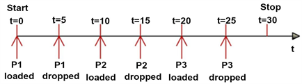
Figure 3. Simulated procedures for the quad-rotor delivering payloads.

Figure 4. Roll angle responses.

Figure 5. Pitch angle responses.

Figure 6. Yaw angle responses.

Figure 7. Estimation of .

Figure 8. Control inputs.

Figure 9. Body rates.
1) The extended state observer can estimate the uncertainties in an accurate manner, significantly enhancing system robustness. The developed predictive controller can degrade influences caused by the sudden change from sudden loading/dropping of payload.
2) Simulation results show that, the developed control scheme is significantly superior to the one based on sliding model control and cascade proportional-integral-derivative, which are commonly used in flight control of quad-rotors.
Acknowledgements
This publication was supported by the Priority Academic Program Development of Jiangsu Higher Education Institutions.
Conflicts of Interest
The author declares no conflicts of interest regarding the publication of this paper.
Cite this paper
Wang, Y. (2019) Predictive Control of Quad-Rotor Delivering Unknown Time-Varying Payloads Based upon Extended State Observer. Advances in Aerospace Science and Technology, 4, 29-41. https://doi.org/10.4236/aast.2019.42003
References
- 1. Gao, P.B., Liu, Y.X., Zhang, H. and Wang, L.L. (2016) Quadrotor Helicopter Attitude Control Using Cascade PID. IEEE Chinese Control and Decision Conference, Yinchuan, 28-30 May 2016, 5158-5163.
- 2. Bouabdallah, S., Noth, A. and Siegwart, R. (2004) PID vs LQ Control Techniques Applied to an Indoor Micro Quadrotor. IEEE/RSJ International Conference on Intelligent Robots and Systems, Sendai, 28 September-2 October 2004, 2451-2456. https://doi.org/10.1109/IROS.2004.1389776
- 3. Zeng, Y., Jiang, Q., Liu, Q. and Jing, H. (2013) PID vs. MRAC Control Techniques Applied to a Quadrotor’s Attitude. IEEE 2nd International Conference on Instrumentation, Measurement, Computer, Communication and Control, Harbin, 8-10 December 2012, 1086-1089. https://doi.org/10.1109/IMCCC.2012.256
- 4. Voos, H. (2009) Nonlinear Control of a Quadrotor Micro-UAV Using Feedback-Linearization. IEEE International Conference on Mechatronics, Malaga, 14-17 April 2009, 1-6. https://doi.org/10.1109/ICMECH.2009.4957154
- 5. Fan, Y.S., Cao, Y.B. and Zhao, Y.S. (2017) Sliding Mode Control for Nonlinear Trajectory Tracking of a Quadrotor. IEEE 36th Chinese Control Conference, Dalian, 26-28 July 2017, 6676-6680. https://doi.org/10.23919/ChiCC.2017.8028413
- 6. Madani, T. and Benallegue, A. (2007) Control of a Quadrotor Mini-Helicopter via Full State Backstepping Technique. Proceedings of the 45th IEEE Conference on Decision and Control, San Diego, CA, 13-15 December 2006, 1515-1520. https://doi.org/10.1109/CDC.2006.377548
- 7. Murray, C.C. and Chu, A.G. (2015) The Flying Sidekick Traveling Salesman Problem: Optimization of Drone-Assisted Parcel Delivery. Transportation Research Part C: Emerging Technologies, 54, 86-109. https://doi.org/10.1016/j.trc.2015.03.005
- 8. Rose, C. (2013) Amazon’s Jeff Bezos Looks to the Future. http://www.cbsnews.com/news/amazons-jeff-bezos-looks-to-the-future/
- 9. Yi, K., Gu, F., Yang, L.L., He, Y.Q. and Han, J.D. (2017) Sliding Mode Control for a Quadrotor Slung Load System. IEEE 36th Chinese Control Conference, Dalian, 26-28 July 2017, 3697-3703.
- 10. Alothman, Y. and Gu, D.B. (2016) Quadrotor Transporting Cable-Suspended Load Using Iterative Linear Quadratic Regulator (iLQR) Optimal Control. IEEE 8th Computer Science and Electronic Engineering, Colchester, 28-30 September 2016, 168-173. https://doi.org/10.1109/CEEC.2016.7835908
- 11. Taylor, C.C. and Engelbrecht, J.A.A. (2017) Acceleration-Based Control of a Quadrotor with a Swinging Payload. 2016 Pattern Recognition Association of South Africa and Robotics and Mechatronics International Conference, Stellenbosch, 30 November-2 December 2016, 1-8. https://doi.org/10.1109/RoboMech.2016.7813188
- 12. Guerrero, M.E., Mercado, D.A., Lozano, R. and Garcia, C.D. (2015) Passivity Based Control for a Quadrotor UAV Transporting a Cable-Suspended Payload with Minimum Swing. 54th IEEE Conference on Decision and Control, Osaka, 15-18 December 2015, 6718-6723. https://doi.org/10.1109/CDC.2015.7403277
- 13. Wang, B., Mu, L.X. and Zhang, Y.M. (2017) Adaptive Robust Control of Quadrotor Helicopter towards Payload Transportation Applications. 36th Chinese Control Conference, Dalian, 26-28 July 2017, 4774-4779. https://doi.org/10.23919/ChiCC.2017.8028107
- 14. Sadeghzadeh, I., Abdolhosseini, M. and Zhang, Y.M. (2014) Payload Drop Application Using an Unmanned Quadrotor Helicopter Based on Gain-Scheduled PID and Model Predictive Control. World Scientific Publishing Company, 2, 39-52. https://doi.org/10.1142/S2301385014500034
- 15. Shastry, A.K., Bhargavapuri, M.T., Kothari, M. and Sahoo, S.R. (2018) Quaternion Based Adaptive Control for Package Delivery Using Variable-Pitch Quadrotors. 2018 Indian Control Conference, Kanpur, India, 4-6 January 2018, 340-345. https://doi.org/10.1109/INDIANCC.2018.8308002
- 16. Pratama, G.N.P., Masngut, I., Cahyadi, A.I. and Herdjunanto, S. (2017) Robustness of PD Control for Transporting Quadrotor with Payload Uncertainties. IEEE 3rd International Conference on Science and Technology-Computer, Yogyakarta, 11-12 July 2017, 11-15. https://doi.org/10.1109/ICSTC.2017.8011844
- 17. Han, J.Q. (2009) From PID to Active Disturbance Rejection Control. IEEE Transactions on Industrial Electronics, 56, 900-906. https://doi.org/10.1109/TIE.2008.2011621
- 18. Zhang, Y., Chen, Z.Q., Zhang, X.H., Sun, Q.L. and Sun, M.W. (2018) A Novel Control Scheme for Quadrotor UAV Based Upon Active Disturbance Rejection Control. Aerospace Science and Technology, 79, 601-609. https://doi.org/10.1016/j.ast.2018.06.017
- 19. Chang, H.Y., Liu, Y.Y., Wang, Y. and Zheng, X.M. (2017) A Modified Nonlinear Dynamic Inversion Method for Attitude Control of UAVs under Persistent Disturbances. IEEE International Conference on Information and Automation, Macau, 18-20 July 2017, 715-721. https://doi.org/10.1109/ICInfA.2017.8078999
- 20. Hou, Z.S., Liu, S.D. and Tian, T.T. (2017) Lazy-Learning-Based Data-Driven Model-Free Adaptive Predictive Control for a Class of Discrete-Time Nonlinear Systems. IEEE Transactions on Neural Networks and Learning Systems, 28, 1914-1928. https://doi.org/10.1109/TNNLS.2016.2561702
- 21. Hou, Z.S. and Jin, S.T. (2013) Model Free Adaptive Control: Theory and Applications. CRC Press, Boca Raton, FL. https://doi.org/10.1201/b15752
- 22. Gao, Z.Q. (2003) Scaling and Bandwidth-Parameterization Based Controller Tuning. Proceedings of the 2003 American Control Conference, Denver, 4-6 June 2003, 4989-4996.