International Journal of Geosciences
Vol.5 No.3(2014), Article ID:44218,10 pages DOI:10.4236/ijg.2014.53026
Quantitative Geomorphometrics for Terrain Characterization
David Coblentz1, Frank Pabian2, Lakshman Prasad3
1EES Division (Geophysics Group), Los Alamos National Laboratory, Los Alamos, USA
2IAT Division (International Research and Analysis), Los Alamos National Laboratory, Los Alamos, USA
3ISR Division (Space Data Systems), Los Alamos National Laboratory, Los Alamos, USA
Email: coblentz@lanl.gov
Copyright © 2014 by authors and Scientific Research Publishing Inc.
This work is licensed under the Creative Commons Attribution International License (CC BY).
http://creativecommons.org/licenses/by/4.0/


Received 17 January 2014; revised 16 February 2014; accepted 9 March 2014
ABSTRACT
The relationship between geology and landforms has long been established with quantitative analysis dating back more than 100 years. The surface expression of various subsurface lithologies motivates our effort to develop an automated terrain classification algorithm based solely on topographic information. The nexus of several factors has recently provided the opportunity to advance our understanding of the relationship between topography and geology within a rigorous quantitative framework, including recent advances in the field of geomorphometrics (the science of quantitative land surface analysis), the availability of very high resolution (sub meter) digital elevation models, and increasing sophisticated geomorphology and image analysis techniques. In the present study, the geological and geomorphological units in an exemplar study area located in Western U.S. (southern Nevada) have been delineated through an evaluation of a high resolution (1-meter and 0.25-meter) digital elevation model. The morphological aspects of these features obtained from DEMs generated from different sources are compared. Our analysis demonstrates that a 1-meter DEM can provide a terrain characterization that can differentiate underlying lithological types and a very high resolution DEM (0.25 meter) can be used to evaluate fracture patterns.
Keywords:Geomorphology; Geomorphometrics; Drainage Patterns; Geologic Characterization; Digital Elevation Models

1. Introduction
The topography of the Earth’s surface provides important information for geomorphic studies because it reflects the interplay between tectonic-associated processes (primarily uplift) and climate erosional processes. Processbased evaluation of geomorphology has established the fact that landforms are not chaotic, but rather are structured by geologic and geomorphic processes over time. Recent advances in the field of geomorphometrics (the science of quantitative land surface analysis) have opened up new opportunities to evaluate the geologic signatures embedded in the topographic fabric of the landscape. In this study, we explore the extent to which geologic information can be extracted from the topography for an exemplar study area by integrating topographic parameters with stream drainage information.
The interplay between the subsurface geology and the surface topography is reflected in the topographic character of the landscape as well as the nature of the drainage pattern formed by the erosion of the topography. The notion that geologic and structural controls (in the form of faults and joint systems) exert a dominant influence on drainage network patterns can be traced back to the late 19th century [1] . There exists a long history in the development of the process-based approach to geomorphology studies [2] with the evaluation of drainage patterns playing a central role in understanding landscape geomorphology [3] -[12] .
While traditional geomorphology research has concentrated on the “forward” problem of evaluating the drainage pattern produced by known geology, there are emerging applications for the “inverse” problem—i.e., predicting the geology from the drainage network and topographic parameters. The central thesis of this approach is that the character of the surface topography and nature of the underlying bedrock geology are intimately related. Early work on this approach was carried out at the Pisgah Crater Test Area (near Barstow, CA) which was extensively studied by NASA as a possible lunar analog for the space program. Studies that sought to correlate the relationship between the topography and underlying geology concluded: “The original hypothesis that surface roughness reflects the geologic nature of rocks appears to be correct” [13] , although the investigators added the caveat that “···it quickly becomes apparent that the scale of sampling required for demonstrating the hypothesis may vary for each area studied” (suggesting the need for high resolution DEMs for accurate site characterization). This approach has also been used extensively for characterizing the geology of the Martian surface [14] -[16] .
In this study, we evaluate the utility of applying the “inverse” approach for generating plausible geologic maps for denied-access sites where only topographic information in the form of digital elevation models (DEMs) is available. At the center of our approach is the exploitation of the fact that the local subsurface geology exerts a primary influence on the drainage pattern of the landscape. Over time, a stream system achieves a particular drainage pattern to its network of stream channels and tributaries as determined by local geologic factors. A quantitative analysis of the forms, density, and texture of the stream channel elements’ network can provide important insight into the underlying geologic, geophysical, and climatic factors that sculpt the landscape.
Topographic data of sufficient resolution relevant to the scale of morphological features that are subject to evaluation are required for this analysis approach. Though 10-m DEMs are widely available in the U.S., they are not always of sufficiently fine scale for lithologic or structure mapping. Thus, we have chosen an exemplar study area with very well documented geology and for which very high resolution DEMs (1-meter and sub-meter resolution) exist in order to fully test our hypothesis that rock type and fracture character can be evaluated with high resolution DEMs. A number of recent studies have demonstrated the utility of high resolution DEMs for quantitative terrain analysis [17] -[20] . This “new generation” of topographic data has resulted in the development of new methodologies for evaluating surface landforms [21] -[25] and has helped to advance our understanding of Earth surface processes [26] -[28] . Furthermore, we have taken advantage of the increasing sophistication of quantitative algorithms for evaluating stream networks [29] -[36] that have been facilitated by the availability of increased memory and computing speed on computational platforms. A 1-meter resolution DEM for a 10 km × 10 km area contains 100 million data cells. Whereas the computation of the drainage network for a region of these size and DEM resolution would have taken a prohibitive amount of computational time only a few years ago, commercial geomorphology analysis tools (such as RiverTools©1) running on modern computing platforms can complete this computation in a small fraction of this time.
In the evaluation presented below, we extend the topography analysis routines of previous investigators [37] -[39] to evaluate the feasibility of differentiating between geologic units and the extent to which the degree of fracture density can be interpreted from an integrated analysis of topographic parameters and drainage patterns. Figure 1 illustrates the differences between the drainage pattern for “soft” rock (alluvium) and “hard”
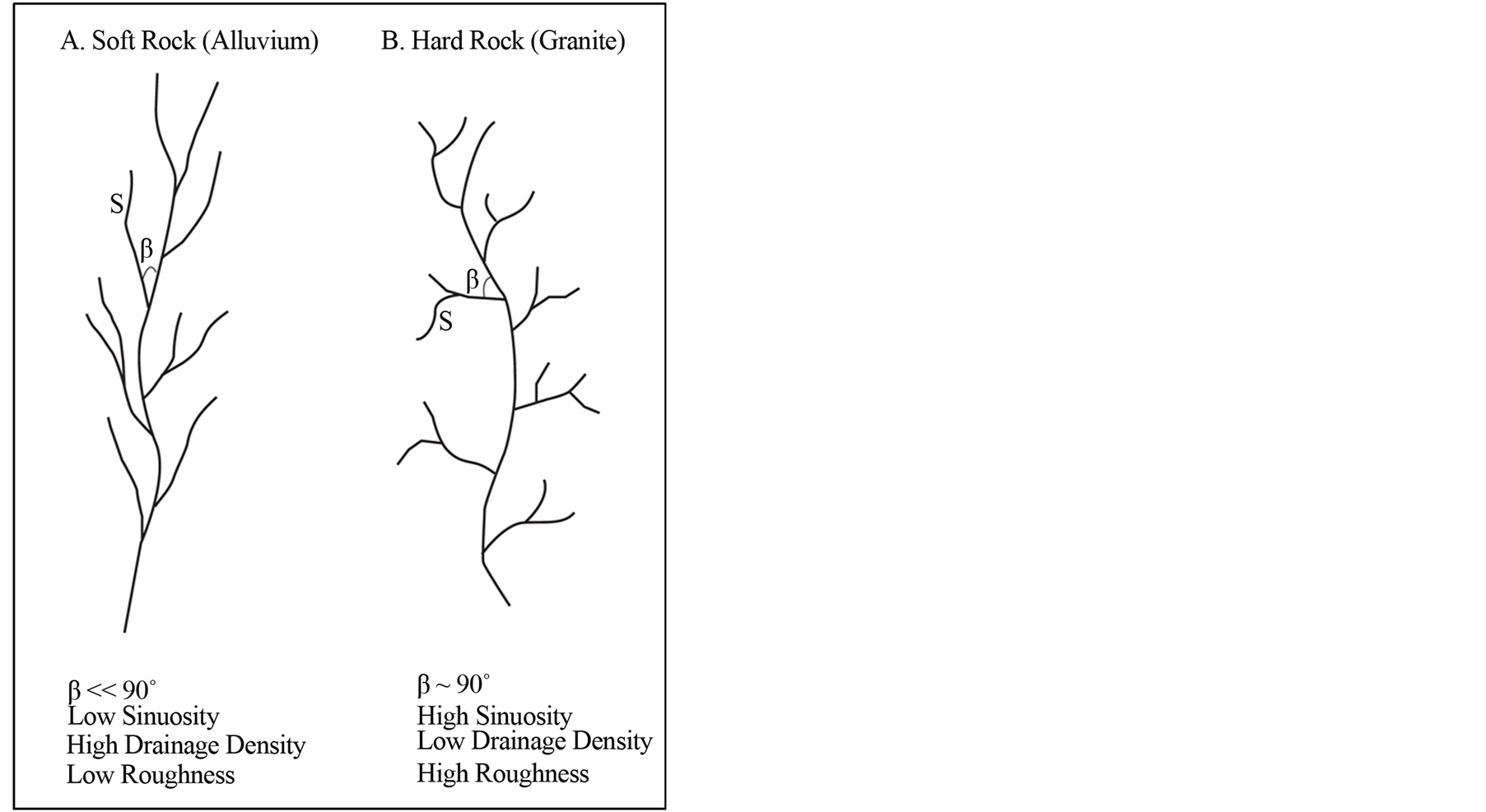
Figure 1. Schematic of the difference in drainage patterns for (A) “soft” rock (alluvium) vs (B) “hard” rock (granite). Harder rock units are characterized by large branch intersection angles (β), high sinuosity, low drainage density and high topographic roughness. This characterization motivates our effort to develop an automated terrain classification algorithm based solely on topographic information.
rock (granite). It is well established that the drainage pattern for the softer alluvium is more linear as opposed to a more dendritic pattern for granite [6] , with lower sinuosity and higher drainage densities for the former. However, the quantitative measurement of how the intersection angle (β in Figure 1) varies between rock types has only recently been addressed [25] . Furthermore, the additional information provided by the integration of drainage pattern character and topographic parameters has not been previously explored (e.g., topographic roughness appears to correlate with sinuosity and inversely with drainage density).
2. Research Objective
The primary aim of this study is to demonstrate local topographic variability for geologic (both lithology and fracture characterization) using a very high resolution DEM. The local topographic variability and terrain characterization is evaluated through a combined quantitative approach that integrates drainage pattern information (i.e., tributary intersection angles, branch sinuosity, and drainage density) with spatial variation in topographic parameters (topographic roughness, organization, and topographic grain). We begin with an overview of the geomorphometric techniques, followed by the application of or methodology for terrain to a 1-meter digital elevation model (DEM) for an exemplar study in southern Nevada (Western U.S.) where the geology is well characterized. At the outset we emphasize that the objective of this study is not so much the development of a technique for precision mapping of geologic units from topographic DEMs, but rather a method for rapid terrain characterization (i.e., “hard” vs. “soft” rock types, prevalent or absent fractures in the bedrock) when the only available information for site assessment is a DEM.
We begin with an overview of geomorphometric techniques and progress to an evaluation of our study area and an assessment of the utility of our approach.
3. Geomorphometrics
Geomorphometry is the science of quantitative land surface analysis “which treats the geometry of the landscape” [40] [41] and uses a quantitative framework for quantifying the character of the land surface [42] -[44] . The field can be further divided into specific geomorphometry, which evaluates discrete surface features and general geomorphometry, which treats the continuous land surface [45] [46] . Our geomorphometric approach is the computer characterization and analysis of continuous topography and falls under the framework of terrain analysis [47] .
3.1. Geomorphic Parameters
A quantitative assessment of the landscape character (e.g., the topographic roughness, organization, and grain orientation) provides the means to evaluate signatures in the surface landscape that may be related to the underlying geology (e.g., rock type, fault and fracture distributions) in the near-surface which can provide site characterization and constraint for geologic framework model development.
Until recently, topographic features have been evaluated with primarily qualitative analysis tools. Parameters such as slope, aspect, and average relief were typically used to categorize the landscape character. The current availability of high speed computing platforms and high-resolution (less than 30 meter spatial resolution) DEMs now provide the opportunity to perform quantitative analyses of topographic surfaces.
In this study, we employ the eigenvalue ratio method [48] [49] to extract the salient geomorphometric parameters from a DEM. If  are a collection of n unit vectors perpendicular to the topographic surfaces described by a DEM, then the orientation matrix T can be formed by the sums of the cross products of the direction cosines [50] -[53] :
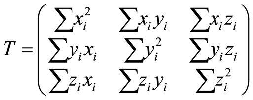 (1)
(1)
The normals to the earth’s surface can be viewed as a cloud of vectors in space and the three eigenvectors define the three dimensional ellipsoid that best models their distribution [49] [54] . The relative magnitudes and orientations of the three eigenvectors of T define the distribution of the surface normals. If the three eigenvalues are normalized with respect to n, then  and
and . For topography the resulting eigenvalues have the following characteristics:
1) The eigenvalue S1 is much greater than S2, and S2 is approximately equal to S3;
2) The eigenvector corresponding to S1 is approximately vertical with the vectors associated with S2 and S3 constrained to the horizontal plane; and 3) S3 points in direction of dominant topographic fabric and provides information about the dominant topographic orientation.
The various ratios of the eigenvectors can be used to define three salient geomorphic parameters: roughness, grain, and organization [55] .
3.1.1. Roughness
In general, roughness can be defined as the irregularity of a topographic surface. It has been noted that roughness cannot be completely defined by a single measure [13] and is more appropriately defined by a “roughness vector”. The eigenvalue ratio method defines roughness as the reciprocal of the flatness or . In general, roughness correlates well with the rugosity and average slope.
3.1.2. Texture and Grain
Topographic grain reflects the degree of linear ridges in the landscape. Originally, it was defined by [47] as “the size of area over which the other factors are to be measured. It is dependent on the spacing of major ridges and valleys and thus indicates texture of topography.” The orientations of S2 and S3 define the dominant grain of the topography.
3.1.3. Topographic Organization
The ratio of S2 to S3 is a measure of the grain strength of the fabric (independent of its orientation). Because there are only two independent eigenvalues (Si), graphs of ln(S1/S2) (“flatness”) and ln(S2/S3) (“organization”) have traditionally been used to evaluate variations in the topographic fabric [49] [54] . The ratio ln(S1/S2) to ln(S2/S3) can be used to evaluate the clustering of the normal vector distribution and was defined as the K-value by [48] . Distributions with K > 1 have vectors that cluster while distributions with K < 1 have distributions which form girdles in a steronet plot [49] . If S1 > S2 and S1 > S3, the orientation data are clustered in a stereographic projection (and are located above the K = 1 axis). Alternatively, if S1 > S3 and S2 > S3, the data form a girdle. Contours of the ratio ln(S1/S3) radiate from the origin and describe the strength of the orientation and thus provides a way to quantify the strength of the topographic grain (with greater strength corresponding to greater grain alignment.)
The utility of the eigenvalue plot has been expanded by its incorporation into DEM analysis software [56] -[59] . This approach has led to the identification of three independent parameters that describe the character of a topographic surface: roughness (which correlates with relief, standard deviation of elevation, average slope, standard deviation of slope, and strength), organization (which expresses the strength of the topographic fabric) via vector drainage network characteristics, (e.g., sinuosity, segment length, element density, and nodal branching angularity) and the average elevation (which correlates poorly with the other topographic parameters.)
The topographic parameters extracted from the DEM using the eigenvalue ratio approach are integrated with additional information extracted from an evaluation of the drainage network.
3.2. Drainage Network Analysis
How a landscape drains and forms drainage networks is a measure of landscape dissection and can provide important information about the underlying rock type and structure. Drainage patterns are considered to be the most important single parameter for quantifying landforms [7] . A drainage network is the pattern formed by streams in a particular drainage basin. The drainage system is dependent on the slope, the nature and attitude of bedrock and on the regional and local fracture pattern. The flow pattern is closely associated with the local geomorphology and as such provides a dense sampling of the surface. The flow pattern contains information about surface structure and material hardness that might give a clue to the local geological substrate. The drainage network influences the geomorphology by erosion and it is this interaction that is a nexus between geology and geomorphology.
Drainage networks are categorized by pattern type, texture, and density and have been classified into six basic types: 1) dendritic, 2) trellis, 3) parallel, 4) radial, 5) annular and 6) rectangular. Their features and occurrence are generalized as follows [7] [60] :
1) Dendritic pattern: a tree-like branching of tributaries join the mainstream at acute angles. Usually this pattern occurs in homogeneous rocks.
2) Trellis pattern: a modification of dendritic, with parallel tributaries converging at nearly right angles. It is indicative of bedrock structure rather than material of bedrock. It can be associated with tilted or interbedded sedimentary rocks, where the main channels follow the strike of beds.
3) Parallel pattern: major tributaries are parallel to major streams and join them at approximately the same angle. It can occur in homogeneous, gentle and uniformly sloping surfaces whose main streams may indicate a fault or fracture zone. Parallel drainage patterns are common in pediment zones and alluvial fans.
4) Radial pattern: a circular network of approximately parallel channels flowing away from a central high point. It usually occurs in volcanoes or domelike structures characterized by resistant bedrock.
5) Annular pattern: a concentric network of channels flowing down and around a central high point. This pattern is usually controlled by layered, jointed and fractured bedrock, in granitic or sedimentary domes.
6) Rectangular pattern: a modification of the dendritic pattern, with tributaries joining mainstream at right angles, forming rectangular shapes. It is controlled by bedrock jointing, foliation and fracturing, indicative of slate, schist, gneiss and resistant sandstone.
At small scales, drainage patterns are thought to reflect the rock fabric [61] . It has long been assumed the relationship occursas a result of zones of weakness in the bedrock enhanced by weathering and erosion processes, although the evaluation of field data has been mostly inconclusive [62] .
The drainage density (defined as the total length of the streams in a drainage basin divided by the total area of the drainage basin [4] ) is a measure of how well or how poorly a watershed is drained by stream channels, and provides important information about the physical characteristics of the drainage basin. Soil permeability (infiltration difficulty) and underlying rock type affect the runoff in a watershed. Rugged regions or those with high relief will also have a higher drainage density than other drainage basins if the other characteristics of the basin are the same.
We turn next to a quantitative evaluation (integrating the topographic and drainage analysis approaches discussed above) of a study area where the geology is well-characterized and very high resolution DEMs of the topography are available.
4. Description of the Exemplar Study Area
The study area (Figure 2) is located in southern Nye County, Nevada in the southern part of the Great Basin region of the Basin and Range Physiographic Province of the Western U.S. The site encompasses an area of 78.5 km2 which is a complex mosaic of geologic units and topographic features. The elevation ranges from 1355 meters to 2165 meters and is characterized by relatively high slopes (average slope = 14˚ ± 10.7˚). The elevations rise steeply to the north and west of the study site where large upland areas are located.
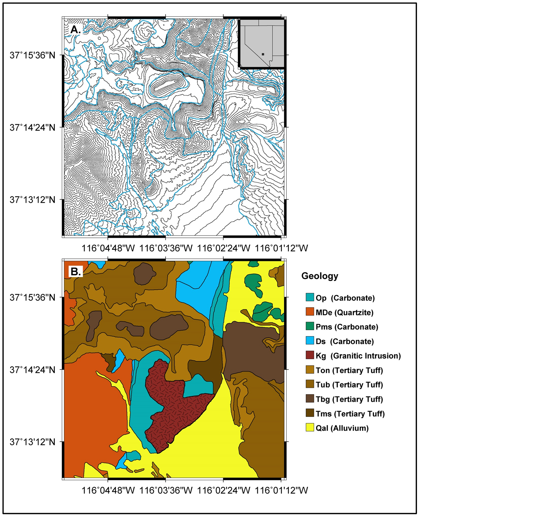
Figure 2. (A) The topography (illustrated with 10 meter contour intervals) and (B) Observed geology for the study area in south-central Nevada. The location was selected based on the well-characterized geology and availability of high-resolution digital elevation models (both 1-meter and 0.25-meter). Of particular interest for this study is the topographic characterization of the granitic intrusion (Kg).
Geology
The geology of the study area is the product of basin-and-range style tectonics. The basins are filled with sedimentary deposits and relatively flat topography, while ranges have higher elevations and are composed of harder Tertiary (volcanic tuff) and pre-Tertiary (Paleozoic) rocks.
The main geologic units in the study area are Tertiary alluvium and sedimentary deposits, Tertiary volcanic tuffs and ash flows, Pre-Tertiary (Paleozoic) carbonate rocks (primarily limestone and dolomites), and intrusive igneous rocks (granites and granodiorites). The Paleozoic rocks are a miogeosynclinal sequence of nearly 4 km of Precambrian to Cambrian clastic deposits (predominantly quartzites) overlain by more than 4 km of Cambrian through Devonian carbonates, 2.5 km of Mississippian argillites and quartzites, and about 1 km of Pennsylvanian to Permian limestones. Following a depositional hiatus during the Mesozoic, Tertiary volcanic rocks of predominantly silicic composition were extruded from numerous eruptive centers during Miocene and Pliocene epochs. Volcanic deposits accumulated to 3 kilometers in total thickness, thinning to extinction outward from the calderas. Extrusion of minor amounts of basalts accompanied Pliocene and Pleistocene filling of structural basins with detritus from the ranges. Granitic intrusion accompanied compressional thrust faulting and folding of Paleozoic sedimentary rocks during regional Laramide-age mountain building. Normal extensional faulting coincided with the outbreak of volcanism during the Miocene and was superimposed on existing Mesozoic structures.
The geologic units of primary interest for this study are shown in Figure 2(B) and a brief description follows. MDe: Eleana Formation (Mississippian and Upper Devonian)—mixture of argillite, siliceous siltstone, quartzite, and conglomerate with a sandy matrix and pebbles and cobbles of chert, quartzite, and argillite; Op: Limestone of the Pogonip Group (Middle and Lower Ordovician)—Moderately resistant, mediumto dark-gray, well bedded, silty limestone, dolomite, and subordinate chert and siltstone. Marked by brownish-orange silt and chert zones; Kg: Intrusive granite of Cretaceous age consisting primarily of granodiorite and porphyritic quartz monzonite. Outcrop area is approximately 4 km2 and it intrudes a sequence of sedimentary rocks of Paleozoic age (limestones, dolomites, and shales), a series of Tertiary volcanic tuffs with various degrees of welded lithology. For the purposes of this study, we examine the properties of one unit is detail (Tub): Tub Spring Tuff (Miocene) —Moderately resistant, gray, tan, and red, partially to densely welded, peralkaline compound ash-flow cooling unit with a total volume estimated to be about 130 km3; Qal: Mixed Quaternary intermediate alluvial deposits (early Holocene and Pleistocene)—Predominantly gravels, sands, and silts.
The granite (Kg) and the limestone (Op) are moderately to highly fractured. The joint density measured in the granites range from 0.52 to 0.89 joints per foot, with two dominant joint patterns: N22˚W and N35˚E.
Many qualitative correlations between the topography and geology are evident in Figure 2, and it is our objective to quantify the correlations with a rigorous geomorphological evaluation.
5. Geomorphometric Analysis
Our geomorphologic analysis is based on a 1-meter resolution DEM that was generated for the study area using a geophysical stereo satellite processing system which exploited the sparse vegetation cover to generate the DEM from 50 cm resolution satellite imagery.
5.1. Topographic Parameters
Figure 3 illustrates the variation in the topographic parameters of roughness and organization for the study area. The “harder” rocks (granite and limestone) are characterized by higher roughness values and moderately higher organization as compared to the “softer” alluvium (which is characterized by low roughness and low organization. A more detailed comparison between the various geologic types is provided by the Flinn Diagram (a plot of “flatness” vs. “organization”) [49] [54] shown in Figure 4. All the lithologies plot in the region with K < 2 (with alluvium K < 5). K values separate readily into “soft” rock (alluvium) with high flatness values (approaching 8), and “hard” rock with flatness values in the range of 3.5 to 4.5. Alluvium exhibits higher strength (S), lower organization, and higher flatness. Limestone (Op) and granite (Kg) are rougher. The harder rocks have about the same S value (strength) and organization. We therefore concur with [13] that topographic roughness is the best parameter for discriminating geologic lithology.
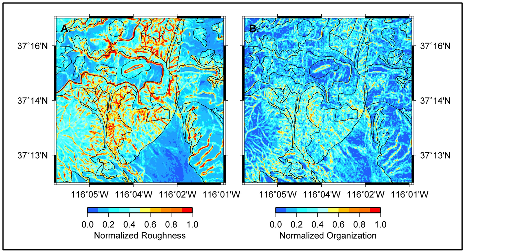
Figure 3. (A) Normalized topographic roughness and (B) Normalized topographic organization for the study area computed using the eigenvalue ration approach described in the text. Both datasets show very good correlation with the geologic boundaries (designated by the black lines).
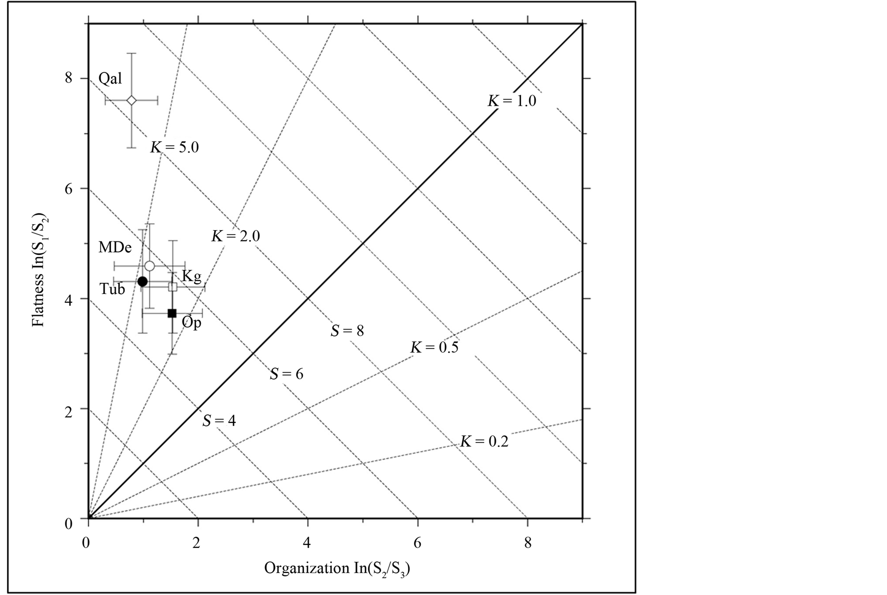
Figure 4. Normalized eigenvalue ratios of directional data for the geologic units of the study area illustrating the relative position in the eigenvalue ratio graph (Flinn diagram). Flatness is a measure of the clustering (coherence) of the topographic surface normals and organization reflects the strength of the topographic fabric. The distance from the origin is controlled by the Strength parameter [ln(S1/S3)] which expresses how strongly the orientation vectors are grouped. Modified from [49] . “Hard” vs. “soft” rock types show a clear separation in the flatness parameter; less so for topographic organization.
5.2. Drainage Pattern Analysis
The drainage pattern computed for the 1-meter DEM is shown in Figure 5. A number of drainage variations correlate with the geologic units shown in Figure 1(b). The change in the drainage pattern between the alluvium (Qal) and the granitic intrusion (Kg) is particularly pronounced. A qualitative assessment of the drainage patterns suggests that the alluvium is characterized by a linear pattern with acute branch intersection angles, while the harder rock types (particularly the granite and limestone) are characterized by dendritic drainage patterns with branch intersection angles closer to 90˚. In the following section, we present a discussion of our drainage analysis routine that provides a way to quantify these qualitative assessments.
The first step in the analysis algorithm is the conversion of the vector drainage network (Figure 5) to a graph of the flow pattern. The graph is a topological reduction of the dense representation of the network into originating flows (branches) that start at a point in the terrain and eventually feed into another at a lower elevation, and continuing flows (trunks) that connect two flow junctions. These branches and trunks constitute the edges of the drainage graph, while flow origination and junction points form the nodes of the graph. For this study area, a 1-meter spatial resolution drainage network with ~2.25 million points was used. We developed an algorithm to reduce this to a drainage graph of ~ 138,000 edges and a similar number of nodes. The graph edges were attributed quantitative structural properties of the stream segments (i.e., branches and trunks) they represent. The structural properties extracted for this study included the node location, stream length, sinuosity (i.e., a measure of how much the stream meandered on its way from one node to another), and direction from one end of the stream segment to the other. We then evaluated the variation of the statistical distributions of these three attributes between the geological regions with the goal of establishing a correlative characterization of the geology through the geomorphology captured by the attributed drainage graph.
In particular, we developed algorithms and software with the following functionality:
1) Compute attributed drainage graphs from drainage networks;
2) Segment distinct drainage catchment areas of the underlying terrain; and 3) Compute attribute distributions for regions of query corresponding to known geological substrates.
This procedure provides the means to query and compare multiple regions using this framework and infer geological correlations and classifications based on the geomorphology.
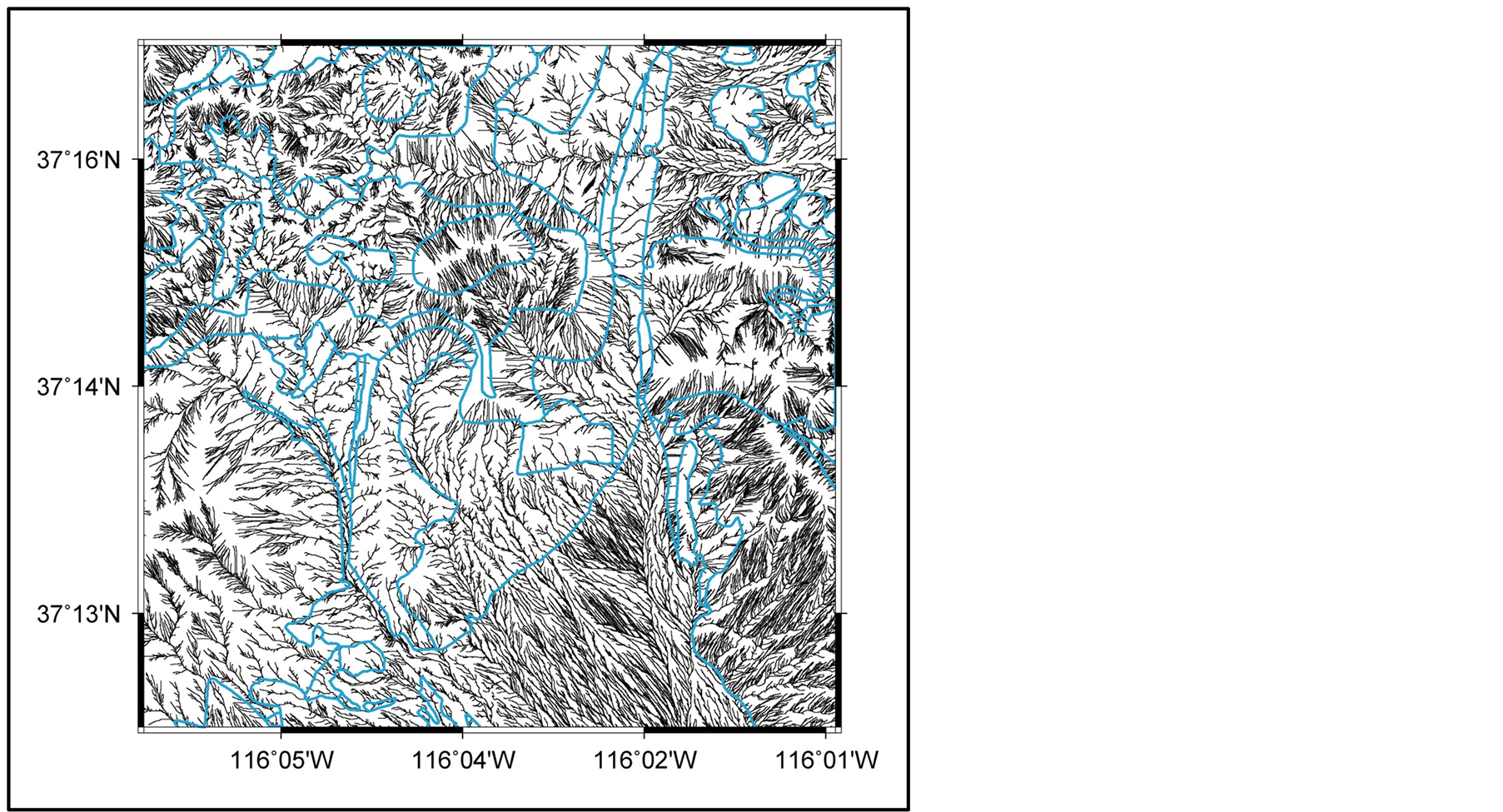
Figure 5. The drainage pattern computed for the 1-meter DEM of the study area (branches shown are limited to Strahler order 4-9 for clarity). The observed geologic units are outlined in blue. Qualitatively, there are distinct differences for the drainage patterns between the various geologic units.
The graph extraction algorithm begins with the drainage network and recasts the point associations as a dense graph. It then computes any cycles in the graph and removes them as they correspond to floodplains and river deltas that are level surfaces of alluvial plains. The resulting graph is made of trees (acyclic graphs) that are disconnected from one another. Each connected tree corresponds to a catchment basin of the terrain. The catchment algorithm then computes these connected components. Next, the graph attribution algorithm computes the topological graph comprised of flow origin and junction points as its only nodes and computes the directional edges connecting these nodes that go from a higher elevation to a lower one by using the DEM. The degrees (number of edges incident upon a node) of the nodes in the dense graph are first computed. The nodes of degree > 2 (i.e., flow junction nodes) are temporarily excluded to get a graph comprising of disconnected edges corresponding to branches and trunks. A connected component analysis is performed to identify nodes corresponding to each edge and the nodes are chained to obtain the flow structure. Attributes of length, sinuosity, and flow direction are computed for each edge using elevation information from the DEM.
Each edge is then represented by its endpoints (i.e., origin and junction nodes for branches, and junction and junction nodes for trunks) in the original dense drainage network graph, while eliminating all other intermediate nodes. Each edge is attributed its length, sinuosity, and direction to obtain an attributed drainage graph. Sinuosity is computed as:
 (2)
(2)
where L is the actual length of the stream segment (branch or trunk) and Ls is the straight-line distance between its end points. This resulted in a ~1:16 reduction in graph size, making the drainage easier to handle computationally, while at the same time creating a higher-level, more informative representation.
5.3. Terrain Characterization
The topographic parameters and drainage characteristics for the four principle geologic units in the study area (Kg, Op, MDe, and Qal) show distinctive difference that can be used to establish a terrain characteristic algorithm for geologic assessment. Histograms of the topographic roughness, the drainage density, stream branch sinuosity and branch intersection angles for the four geologic units in the study area (Figure 6) support the following generalities:
1) Harder rock types (granite and limestone) are characterized by rougher topography, lower drainage densities, higher sinuosity, and high angle branch intersections; 2) “Softer” alluvium is characterized by smoother topography, higher drainage densities, lower sinuosity, and lower branch intersection angles; 3) The quartzite/conglomerate Eleana Formation (MDe) has an intermediate terrain character to the hard and soft rock units; and 4) Both roughness and sinuosity are negatively correlated with drainage density (R-squared value for a plot of the mean values is of nearly 90% for both distributions) (averages and one standard deviation about the mean are listed in Table 1).
The difference between the branch-to-trunk angles and trunk-to-trunk angles for the alluvium vs. granite is illustrated in the histogram shown in Figure 6(E). The bimodality of the angle distribution corresponds to the two subcategories. For geologic types, the left peak corresponds to the branch-to-trunk distribution, while the right peak corresponds to the trunk-to-trunk angle distribution. In the case of granite, the two peaks in the histogram have a smaller angle separation reflecting the fact that branch-to-trunk angles are less acute and branch-to-branch

Table 1. Average values for terrain parametersa.
aAverage ± one standard deviation for terrain parameters plotted in the histograms shown in Figure 6.
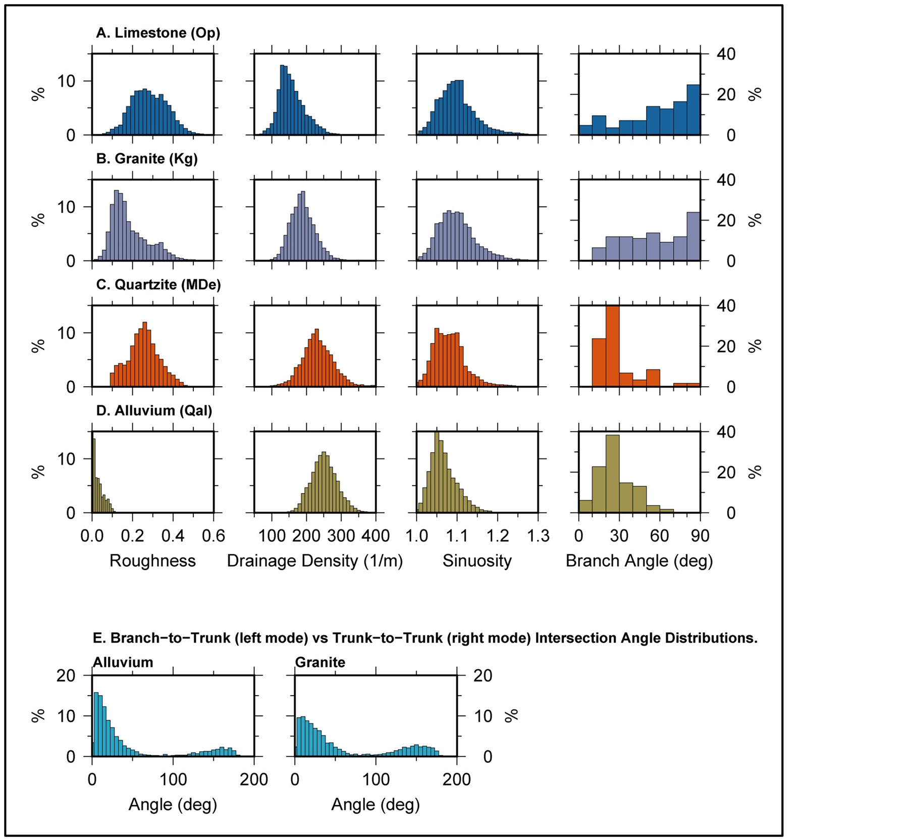
Figure 6. Histograms (percentage contribution) for the topographic roughness, drainage density, branch sinuosity, and branch intersection angles for (A) intrusive granite (Kg), (B) limestone (Op), (C) quartzite (MDe) and (D) alluvium (Qal) lithologic units within the study area. The mean values for the distributions are listed in Table 1. The various geologic units have distinctive distribution for these four parameters, motivating their inclusion into the terrain characterization algorithm. The difference between the branch-to-trunk angles and trunk-to-trunk angles for the alluvium vs. granite is shown in (E). The bimodality of the angle distribution corresponds to the two subcategories. The left peak is branch-to-trunk distribution, while the right peak is trunk-to-trunk angle distribution. In the case of granite, these peaks are closer to each other (since branch-to-trunk angles are less acute and branchto-branch angles are less obtuse) than in the case of alluvium (since branch-to-trunk angles are more acute and trunk-to-trunk angles are more obtuse).
angles are less obtuse. The converse is true for alluvium; where branch-to-trunk angles are more acute and trunk-to-trunk angles are more obtuse).
Exploiting the strong correlation between the geology and the geomorphometric parameters, we next developed an algorithm to calculate a Terrain Characterization Type (TCT) value which integrates the roughness, drainage density and sinuosity. Each of the three parameters was binned into a high, medium and low category based on the mean values ± one standard deviation about the mean. In aggregate, this yields 27 terrain characterization types.
The validity of this approach was assessed by computing the predicted TCT value for the known geologic rock types. Histograms of the predicted terrain types for five geologic types (Figure 7) shows that the geologic
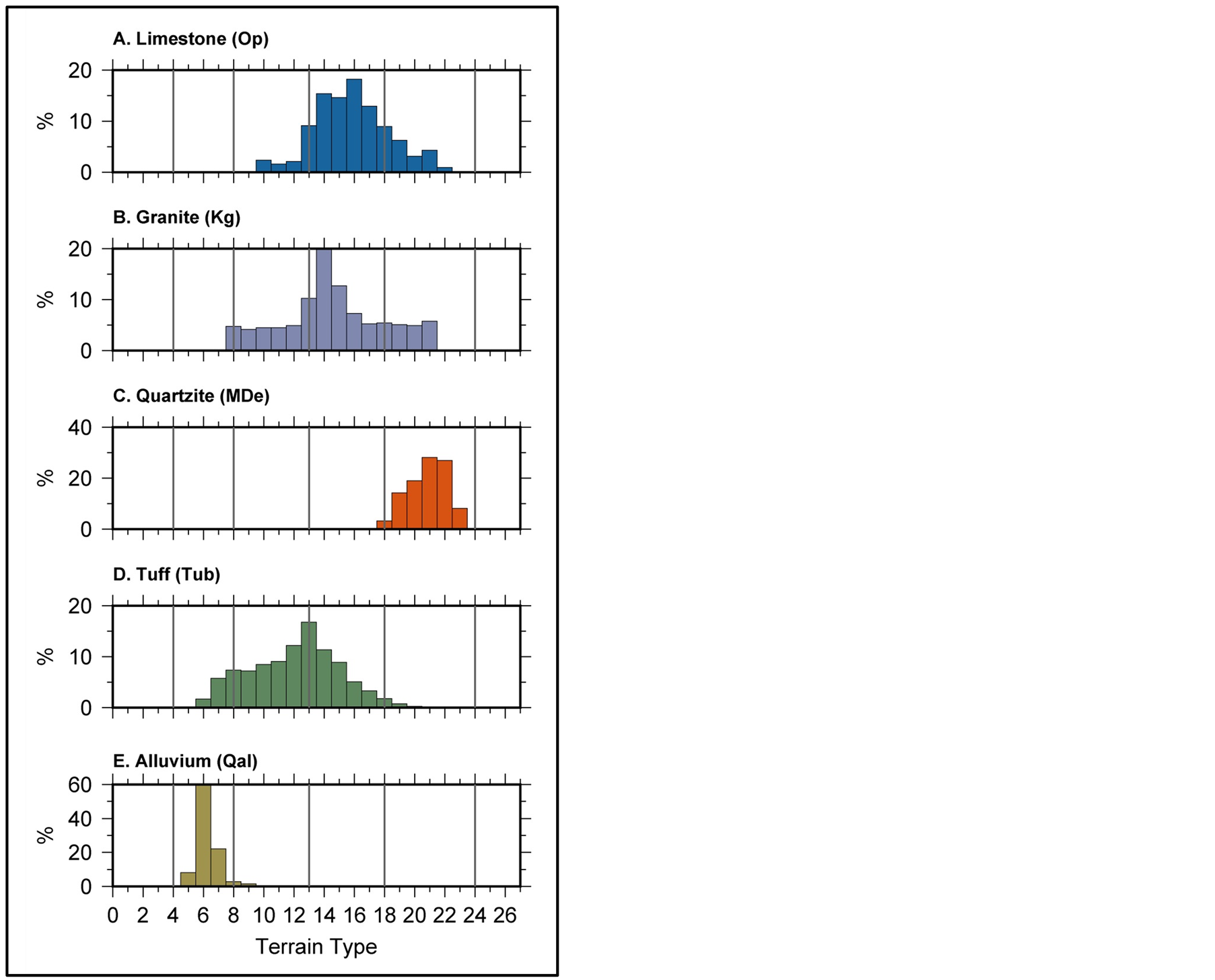
Figure 7. Histograms for the predicted terrain type (TCT) values for five geologic units: the intrusive granite (Kg), limestone (Op), quartzite (MDe), Tub Spring Tuff (Tub), and alluvium (Qal). Vertical bars designate the differentiating terrain type limits for the five lithological units evaluated.
units indeed separate into distinct TCT zones: low values (4 - 8) for alluvium; tuffs (Tub) in the range (8 - 13); the “hard” granite (Kg) and limestone (Op) both fall in the range of 14 - 18; and the quartzite/conglomerate Eleana Formation (MDe) is characterized by high TCT values in the range of 19 - 24. Applying the TCT algorithm to the entire study area yields a predicted terrain type map (Figure 8) which is in excellent agreement with the observed geologic units shown in Figure 1(a). This illustrates that predicting geology is possible with a high resolution DEM, binned at the resolution of the DEM and then smoothed with a 3 × 3 window.
5.4. Fracture Characterization
The analysis of geomorphic characteristics that can be used for fracture characterization requires sub-meter DEMs that can capture features of the same spatial order as the fracture separation.
Recently, significant progress has been made in the application of laser scanning for terrain characterization. Both Terrestrial Laser Scanner (TLS) and Airborne Laser Swath Mapping technology (ALSM), using LiDAR (Light Detection And Ranging) technology, now provide high resolution topographic data with notable advantages over traditional survey techniques. A valuable characteristic of these technologies is their capability to produce sub-meter resolution Digital Terrain Models (DTMs), and high-quality land cover information (Digital Surface Models, DSMs) over large areas. In particular, it has been demonstrated that the geometric characteristics of discontinuities (such as fractures) including orientation, spacing, persistence and roughness can be obtained using the analysis of LiDAR data [63] -[66] .
A second method for predicting fracture distribution and orientation is the evaluation of the topographic curvature [67] , which can be used to predict areas of high fracture density as well as the orientation of fractures that formed during deformation of strata. In general, geologic strata with high Gaussian curvature can be expected to correspond with zones of greater deformation and higher density of fractures [68] . Furthermore, there is a clear relationship between fracture permeability and curvature [69] , and fracture porosity has been related to the product of bed thickness and curvature. Other studies have shown that zones of high fracture density coincide with areas of elevated curvature [70] -[73] , a notion that is supported by the results of numerical modeling [74] -[80] .
In this study we evaluate a 0.25-meter DEM (collected using an airborne LiDAR platform) for a 7 km2 subregion of the study area which includes parts of the granite (Kg), limestone (Op) and alluvium lithology (Qal) in the southern part of the study area. Our primary objective is to evaluate the extent to which fracture orientations can be extracted from a very high resolution DEM through an integrated analysis of the curvature and topographic grain information. The granite intrusion (Kg, Figure 1) is moderately to highly fractured; with two dominant joint patterns (N22˚W and N35˚E) that are well-documented and provide constraint for our analysis [75] [76] .
We begin by testing the hypothesis that the topographic grain extracted from a very high resolution DEM correlates with the local fracture orientation. The topographic grain was extracted for an analysis window centered on a site in the granitic intrusion of known fracture orientation. Figure 9 illustrates the variation in the topographic grain orientation as a function of analysis window size (from 2 to 25 meters). With the exception of very small window size (2 and 3 meters) the grain orientation is remarkably consistent with dominant joint orientations of N35˚E. This result suggests that a map of the topographic grain orientation can be used to estimate fracture orientations for a larger scale.
In Figure 10 we combine the topographic grain orientation with a map of the Laplacian curvature to construct a proxy map of the fracture density and orientation for the sub-region of the study area. Highest fracture densities are predicted for the limestone and granitic lithologies (which is confirmed by observation). We note, how-
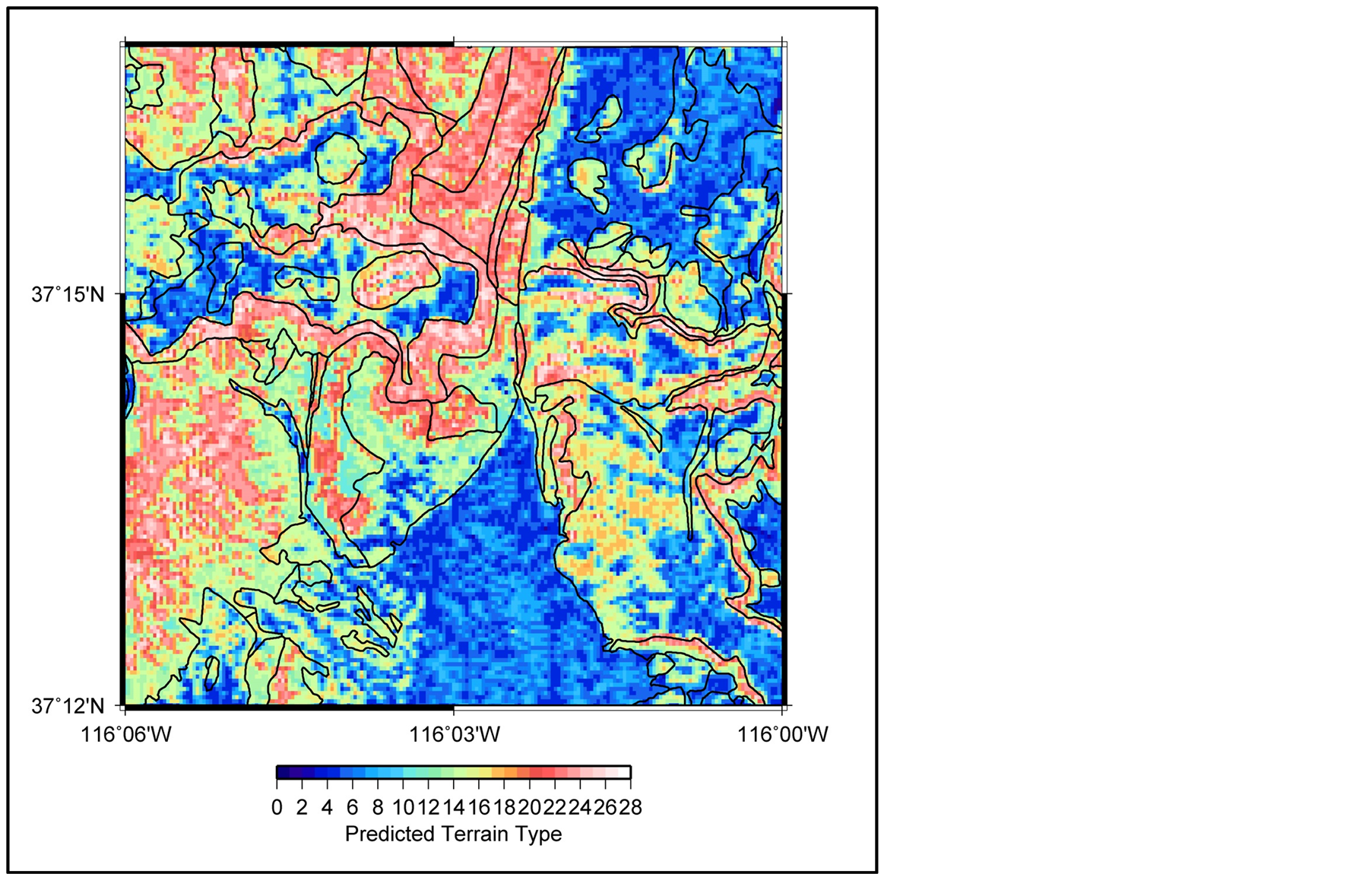
Figure 8. Predicted terrain type (TCT) values computer at a 10-meter resolution for study area using the differentiating terrain type limits discussed in Figure 7. The five lithological units evaluated show quantifiable spatial distinction in the predicted terrain type.
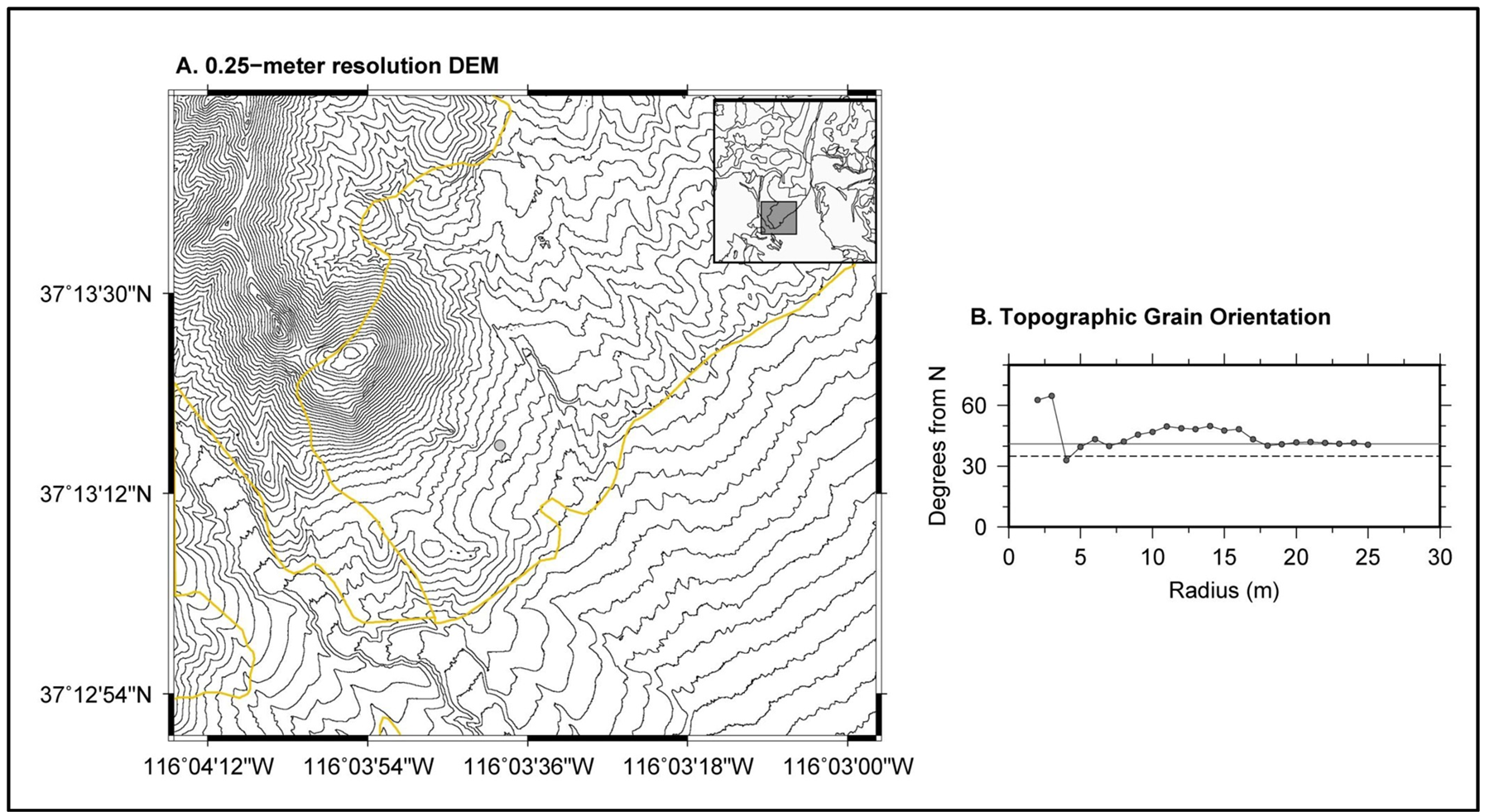
Figure 9. (A) Contoured topography (2-meter contour intervals) for the 0.25-meter DEM of the subregion (gray area on the inset map). Grey-filled circle designates the location of the measured fracture orientation. (B) Variation in the topographic grain orientation (computed using the eigenvalue ratio approach discussed in the text) for an analysis window with radius between 2- and 25-meters. Black dash line designates one of the dominant fracture orientations for the site (N35oE); gray line indicates the average for the computed topographic grain (N41˚E).
ever, that a number of cultural artifacts (primarily road and ground excavation scars) are evident in Figure 10. We readily acknowledge that correlation does not prove causality and further work is needed to develop a deterministic model for predicting fracture patterns in geology. We also acknowledge that it is well recognized that fracture intensities do not correlate directly with curvature since curvature is only one mechanism for fracture development (other mechanisms include stretching, faulting, bedding-plane slip, the influence of preexisting fractures, and tectonic loading) [76] . Nevertheless, the close correlations between the topographic grain and the observed fracture patterns for the granite intrusion considered here is intriguing.
6. Discussion
The relationship between geology and landforms has long been established, with a history extending back more than 100 years [77] [78] . The character of the Earth’s topography is the product of competing elements of constructive (e.g., plate tectonics, volcanic eruptions and sedimentation), and degradational processes (e.g., chemical and mechanical weathering, erosion and subsidence). Variations in the mechanical and chemical properties of geologic formations allow variable weathering which results in the exposure and highlight of near-surface structures. These structural imprints are recorded in DEMs of the topography and, as we have demonstrated above, the quantitative analysis of the landscape can provide valuable insight into the geology of the underlying bedrock. Indeed, much of our understanding of planetary geology is derived from the analysis and interpretation of extraterrestrial landforms and landform interrelationships [79] [81] . Clearly, our understanding earth surface processes relies on modern digital terrain representations which in turn depend strongly on the quality of the topographic data. In the last decade, a range of new remote sensing techniques has led to a dramatic increase in terrain information. Here, we have sought to demonstrate that analysis of meterto sub-meter scale DEMs can provide terrestrial geologic information that can supplement field mapping and other types of remote-sensing surveys.
There are a number of applications that call for the methodology presented in this study. The development of high-fidelity geologic framework models for denied-access sites that maximize the available information about the subsurface is a challenging undertaking but one with important global security application. Typical geologic settings very complex with many features (e.g., intrusions, faults and fractures) that exert influence on many
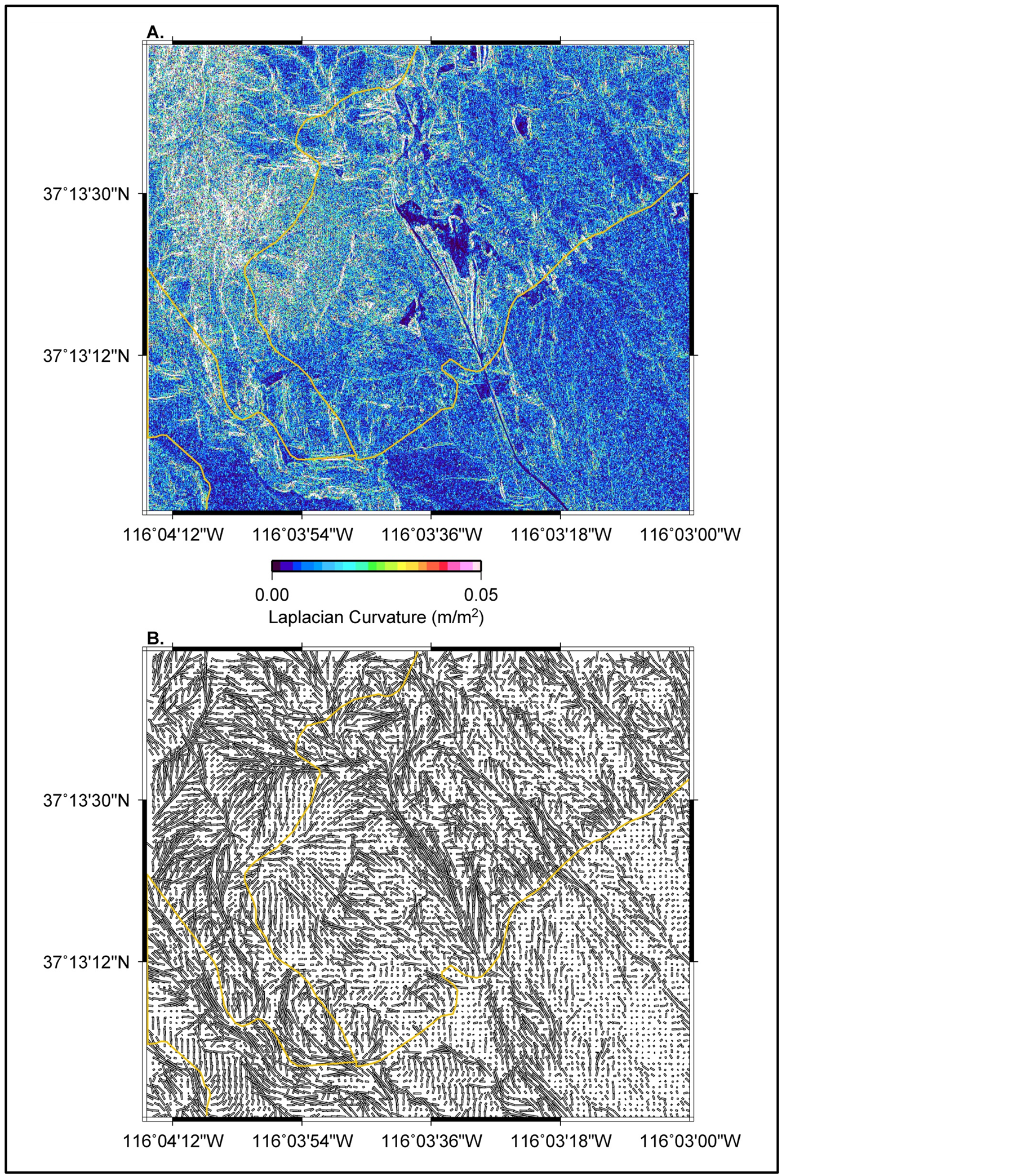
Figure 10. (A) Absolute value of the Laplacian curvature of the 0.25-meter DEM. Yellow lines designate observed geologic boundaries. High curvature values define regions of predicted high fracture density (as discussed in the text), with lighter color values corresponding to regions of high fracture density. Several cultural artifacts (e.g., excavation scars, roads and pipelines) also produce high curvature values that should be considered as cultural noise. (B) The orientation of the topographic grain (computed for at a 50-meter resolution) which is interpreted as a proxy for the fracture orientation (see discussion in the text).
geodynamics processes. Currently, the geologic characterization of denied-access sites is limited to very simplistic representations of the subsurface geology (e.g., either half-space or planar geologic layers). This is a critical shortcoming given that many proliferation detection applications could benefit from more comprehensive 3-d models of the subsurface geology (e.g., the modeling of seismic wave propagation and potential leakage pathways of radio-nuclides through rock fractures, as well as apriori site characterization and evaluation for treaty monitoring.) A need exists for the development of techniques to provide site characterization information for denied-access sites using readily available remote-sensing data (in particular, topographic data) which is available on a global basis at very high spatial resolution [82] .
7. Conclusions
Given the limitations and caveats discussed above, we draw the following general conclusions from our study:
Topography can reflect the geological structure of a terrain, supporting the conclusions of [83] -[91] that geology can be derived from topography. Indeed, our results support the conclusion “···Topography is an expression, by means of physical features, not only of the geology of a country, but to a very large extent of its geological history. So much is this so that if on a map the geology and topography do not fit snugly together either one or the other is wrongly mapped” [83] .
We find that a DEM with a resolution of at least 1-meter is required for differentiation of geologic lithologies through evaluation of the topography. Geologic units ranging from soft alluvium, intermediate tuffs, and hard granite and limestone can be differentiated with high resolution (sub-meter) DEM.
Mapping and characterization of the fracture patterns and densities require a sub-meter resolution DEM. Close correlations between topographic grain and observed fracture patterns for a granite intrusion considered here provide a first step in establishing sub 1m DEM (0.25 m) as a predictive tool for characterization of fracture patterns.
Traditionally, geological maps were prepared from conventional ground surveys based on field observations conducted along traverse lines at regular intervals. Remote sensing techniques have opened a new era in mapping lithology, particularly for denied-access sites. In this study, we have demonstrated the feasibility of constructing a plausible first-order geoloigc map based solely on topographic data. Improvements to our approach would include the integration and evaluate of hyperspectral image data which could provide additional lithological information. Inclusion of this additional information could provide structural constraint that could inform the development of a 3-D geologic framework models.
Acknowledgements
Constructive conversations with Brian Crone and Dale Anderson on the methodology present in this study led to a number of improvements in the manuscript. The authors wish to express their gratitude to the National Nuclear Security Administration, Defense Nuclear Nonproliferation Research and Development (DNN R&D), and the Source Physics Experiment working group, a multi-institutional and interdisciplinary group of scientists and engineers. This work was conducted by Los Alamos National Laboratory under award number DE-AC52- 06NA25946. This geomorphometric algorithm developmental study for remote sensing-based geologic mapping was partially supported by LANL LDRD Reserve Funding. Key insights for this work were derived in the course of a recent advanced geological site characterization conducted under the auspices of the U.S. State Department’s Office of Verification and Transparency Technologies. This manuscript is Los Alamos Publication LA-UR-14-2005.
References
- Kinahan, G.H. (1875) Valleys and Their Relationship to Fractures, Fissures, and Faults. Trubner, London. http://dx.doi.org/10.5962/bhl.title.23043
- Burt, T.P., Chorley, R.J., Brunsden, D., Cox, N. and Goudie, A.S. (2008) The History of the Study of Landforms or the Development of Geomorphology Volume 4: Quaternary and Recent Processes and Forms (1890-1965) and the MidCentury. The Geological Society of London, London, 1056 p.
- Zernitz, E.R. (1932) Drainage Patterns and Their Significance. Journal of Geology, 40, 498-521. http://dx.doi.org/10.1086/623976
- Horton, R.E. (1945) Erosional Development of Streams and Their Drainage Basins: Hydrophysical Approach to Quantitative Morphology. Geological Society of America Bulletin, 56, 275-370. http://dx.doi.org/10.1130/0016-7606(1945)56[275:EDOSAT]2.0.CO;2
- Melton, M.A. (1958) Correlation Structures of Morphometric Properties of Drainage Systems and Their Controlling Agents. Journal of Geology, 66, 442-460. http://dx.doi.org/10.1086/626527
- Howard, A.D. (1967) Drainage Analysis in Geologic Interpretation: A Summation. American Association of Petroleum Geologist Bulletin, 51, 2246-2259.
- Way, D.S. (1973) Terrain Analysis. Dowden Hutchinson and Ross, Stroudsburg, 400 p.
- Jarvis, R.S. (1977) Drainage Network Analysis. Progress in Physical Geography, 1, 271-295. http://dx.doi.org/10.1177/030913337700100203
- Unwin, D.J. (1977) Statistical Methods in Physical Geography. Progress in Physical Geography, 1, 185-221. http://dx.doi.org/10.1177/030913337700100201
- Abrahams, A.D. (1984) Channel Networks: A Geomorphological Perspective. Water Resources Research, 20, 161-188. http://dx.doi.org/10.1029/WR020i002p00161
- Pike, R.J., Evans, I.S. and Hengl, T. (2009) Chapter 1 Geomorphometry: A Brief Guide. In: Hengl, T. and Reuter, H.I., Eds., Developments in Soil Science, Elsevier, 33, 3-30. http://dx.doi.org/10.1016/S0166-2481(08)00001-9
- Pike, R.J. (2002) A Bibliography of Terrain Modeling (Geomorphometry), the Quantitative Representation of Topography-Supplement 4.0. US Geological Society Open File Report 02-465, 158 p.
- Hobson, R.D. (1972) Surface Roughness in Topography: A Quantitative Approach. In: Chorley, R.J., Ed., Spatial Analysis in Geomorphology, Methuen & Co., London, 221-245.
- Smith, D.E., Zuber, M.T., Solomon, S.C., Phillips, R.J., Head, J.W., Garvin, J.B., Banerdt, W.B., Muhleman, D.O., Pettengill, G.H., Neumann, G.A., Lemoine, F.G., Abshire, J.B., Aharonson, O., Brown, C.D., Hauck, S.A., Ivanov, A.B., McGovern, P.J., Zwally, H.J. and Duxbury, T.C. (1999) The Global Topography of Mars and Implications for Surface Evolution. Science, 284, 1495-1503. http://dx.doi.org/10.1126/science.284.5419.1495
- Shepard, M.K., Campbell, B.A., Bulmer, M.H., Farr, T.G., Gaddis, L.R. and Plaut, J.J. (2012) The Roughness of Natural Terrain: A Planetary and Remote Sensing Perspective. Journal of Geophysical Research, 106, 32777-32795. http://dx.doi.org/10.1029/2000JE001429
- Goetz, A.F.H. and Rowan, L.C. (1981) Geologic Remote Sensing. Science, 211, 781-791. http://dx.doi.org/10.1126/science.211.4484.781
- Glenn, N.F., Streutker, D.R., Chadwick, D.J., Thackray, G.D. and Dorsch, S.J. (2006) Analysis of LiDAR-Derived Topographic Information for Characterizing and Differentiating Landslide Morphology and Activity. Geomorphology, 73, 131-148. http://dx.doi.org/10.1016/j.geomorph.2005.07.006
- Slatton, K.C., Carter, W.E., Shrestha, R.L. and Dietrich, W.E. (2007) Airborne Laser Swath Mapping: Achieving the Resolution and Accuracy Required for Geosurficial Research. Geophysical Research Letters, 34, Article ID: L23S10. http://dx.doi.org/10.1029/2007GL031939
- Tarolli, P., Arrowsmith, J.R. and Vivoni, E.R. (2009) Understanding Earth Surface Processes from Remotely Sensed Digital Terrain Models. Geomorphology, 113, 1-3. http://dx.doi.org/10.1016/j.geomorph.2009.07.005
- Cavalli, M. (2013) Introduction to the Special Issue: High Resolution Topography, Quantitative Analysis and Geomorphological Mapping. European Journal of Remote Sensing, 46, 60-64. http://dx.doi.org/10.5721/EuJRS20134604
- Zevenbergen, L.W. and Thorne, C.R. (1987) Quantitative Analysis of Land Surface Topography. Earth Surface Processes and Landforms, 12, 47-56. http://dx.doi.org/10.1002/esp.3290120107
- Arrowsmith, J.R. and Zielke, O. (2009) Tectonic Geomorphology of the San Andreas Fault Zone from High Resolution Topography: An Example from the Cholame Segment. Geomorphology, 113, 70-81. http://dx.doi.org/10.1016/j.geomorph.2009.01.002
- Trevisani, S., Cavalli, M. and Marchi, L. (2012) Surface Texture Analysis of a High-Resolution DTM: Interpreting an Alpine Basin. Geomorphology, 161-162, 26-39. http://dx.doi.org/10.1016/j.geomorph.2012.03.031
- Cazorzi, F., Fontana Dalla, G., De Luca, A., Sofia, G. and Tarolli, P. (2013) Drainage Network Detection and Assessment of Network Storage Capacity in Agrarian Landscape. Hydrological Processes, 27, 541-553. http://dx.doi.org/10.1002/hyp.9224
- Pike, R.J. (2000) Geomorphometry—Diversity in Quantitative Surface Analysis. Progress in Physical Geography, 24, 1-20.
- Coblentz, D. and Karlstrom, K.E. (2011) Tectonic Geomorphometrics of the Western United States: Speculations on the Surface Expression of Upper Mantle Processes. Geochemisty, Geophysics, Geosystems, 12, Article ID: Q11002. http://dx.doi.org/10.1029/2011GC003579
- Tarolli, P. and Dalla Fontana, G. (2009) Hillslope to Valley Transition Morphology: New Opportunities from High Resolution DTMs. Geomorphology, 113, 47-56. http://dx.doi.org/10.1016/j.geomorph.2009.02.006
- Deng, Y.X. (2007) New Trends in Digital Terrain Analysis: Landform Definition, Representation, and Classification. Progress in Physical Geography, 31, 405-419. http://dx.doi.org/10.1177/0309133307081291
- Pike, R.J. (1988) The Geometric Signature: Quantifying Landslide-Terrain Types from Digital Elevation Models. Mathematical Geology, 20, 491-505. http://dx.doi.org/10.1007/BF00890333
- O’Callaghan, J.F. and Mark, D.M. (1984) The Extraction of Drainage Networks from Digital Elevation Data. Computer Vision, Graphics, and Image Processing, 28, 323-344. http://dx.doi.org/10.1016/S0734-189X(84)80011-0
- Mark, D.M. (1984) Automated Detection of Drainage Network from Digital Elevation Model. Cartographica, 21, 168-178. http://dx.doi.org/10.3138/10LM-4435-6310-251R
- Chorowicz, J., Ichoku, C., Riazanoff, S., Kim, Y.J. and Cervelle, B. (1992) A Combined Algorithm for Automated Drainage Network Extraction. Water Resources Research, 28, 1293-1302. http://dx.doi.org/10.1029/91WR03098
- Chorowicz, J., Kim, J., Manoussis, S., Rudant, J.P., Foin, P. and Veillet, I. (1989) A New Technique for Recognition of Geological and Geomorphological Patterns in Digital Terrain Models. Remote Sensing of Environment, 29, 229-239. http://dx.doi.org/10.1016/0034-4257(89)90002-3
- Strahler, A.N. (1992) Quantiative/Dynamic Geomorphology at Columbia 1945-1960: A Retrospective. Progress in Physical Geography, 16, 65-84. http://dx.doi.org/10.1177/030913339201600102
- Murray, A.B. and Paoloa, C. (1996) A New Quantitative Test of Geomorphic Models, Applied to a Model of Braided Streams. Water Resources Research, 32, 2579-2587. http://dx.doi.org/10.1029/96WR00604
- Tucker, G.E., Catani, F., Rinaldo, A. and Bras, R.L. (2001) Statistical Analysis of Drainage Density from Digital Terrain Data. Geomorphology, 36, 187-202. http://dx.doi.org/10.1016/S0169-555X(00)00056-8
- Zhang, L. and Guilbert, E. (2013) Automatic Drainage Pattern Recognition in River Networks. International Journal of Geographical Information Science, 27, 2319-2342. http://dx.doi.org/10.1080/13658816.2013.802794
- Tribe, A. (1992) Automated Recognition of Valley Lines and Drainage Networks from Grid Digital Elevation Models: A Review and a New Method. Journal of Hydrology, 139, 263-293.
- Schmid-McGibbon, G. (1995) Generalization of Digital Terrain Models for Use in Landform Mapping. Cartographica, 32, 26-38. http://dx.doi.org/10.3138/R753-0776-2767-R452
- Chorley, R.J., Malm, D. and Pogorzelski, H.A. (1957) A New Standard for Estimating Drainage Basin Shape. American Journal of Science, 255, 138-141. http://dx.doi.org/10.2475/ajs.255.2.138
- Chorley, R.J. (1957) Climate and Morphometry. Journal of Geology, 65, 628-638. http://dx.doi.org/10.1086/626468
- Wood, W.F. and Snell, J.B. (1960) A Quantitative System for Classifying Landforms. Quartermaster Research & Engineering Command, U.S. Army Technical Report, EP-124.
- Pike, R.J., Evans, I. and Hengl, T. (2008) Geomorphometry: A Brief Guide. In: Hengl, T. and Reuter, H.I., Eds., Geomorphometry—Concepts, Software, Applications, Series Developments in Soil Science, Vol. 33, Elsevier, Amsterdam, 3-33.
- Rasemann, J., Schmidt, L., Schrott, R. and Dikau, R. (2004) Geomorphometry in Mountain Terrain. In: Bishop, M. and Shroder, J.F., Eds., Geographic Information Science in Mountain Terrain, Springer, Heidelberg, 101-145.
- Evans, S. (1972) General Geomorphometry, Derivatives of Altitude, and Descriptive Statistics. In: Chorley, R.J., Ed., Spatial Analysis in Geomorphology, Methuen & Co. Ltd., London, 17-90.
- Thorn, C.E. (1988) An Introduction to Theoretical Geomorphology. Unwin Hyman, Boston, 247 p. http://dx.doi.org/10.1007/978-94-010-9441-2
- Wilson, J.P. and Gallant, J.C. (2000) Terrain Analysis: Principles and Applications. John Wiley and Sons, New York, 479 p.
- Chapman, C.A. (1952) A New Quantitative Method of Topographic Analysis. American Journal of Science, 250, 428- 452. http://dx.doi.org/10.2475/ajs.250.6.428
- Woodcock, N.H. (1977) Specification of Fabric Shapes Using an Eigenvalue Method. Geological Society of America Bulletin, 88, 1231-1236. http://dx.doi.org/10.1130/0016-7606(1977)88<1231:SOFSUA>2.0.CO;2
- Fara, H.D. and Scheiddegger, A.E. (1963) An Eigenvalue Method for the Statistical Evaluation of Fault Plane Solutions of Earthquakes. Bulletin of the Seismological Society of America, 53, 811-816.
- Fisher, H.L., Lewis, T. and Embleton, B.J.J. (1987) Statistical Analysis of Spherical Data. Cambridge University Press, Cambridge, 344 p. http://dx.doi.org/10.1017/CBO9780511623059
- Scheiddegger, A.E. (1965) On the Statistics of the Orientation of Bedding Planes, Grain Axes, and Similar Sedimentological Data. U.S. Geological Society Professional Paper, 525-C, 164-167.
- Watson, G.S. (1966) Statistics of Orientation Data. Journal of Geology, 74, 786-795. http://dx.doi.org/10.1086/627211
- Woodcock, N.H. and Naylor, M.A. (1983) Randomness Testing in 3-Dimensional Orientation Data. Journal of Structural Geology, 5, 539-548. http://dx.doi.org/10.1016/0191-8141(83)90058-5
- Mark, D.M. (1975) Geomorphometric Parameters: A Review and Evaluation. Geografiska Annaler. Series A, 57, 165- 177. http://dx.doi.org/10.2307/520612
- Guth, P. (1999) Quantifying Topographic Fabric: Eigenvector Analysis Using Digital Elevation Models. Advances in Computer-Assisted Recognition, 3584, 233-241. http://dx.doi.org/10.1117/12.339825
- Guth, P. (1999) Quantifying and Visualizing Terrain Fabric from Digital Elevation Models. 4th International Conference on GeoComputation, Mary Washington College Fredericksburg, Virginia. http://www.geocomputation.org/1999/096/gc_096.htm
- Guth, P., Ressler, E.K. and Bacastow, T.S. (1987) Microcomputer Program for Manipulating Large Digital Terrain Models. Computers and Geosciences, 13, 209-213. http://dx.doi.org/10.1016/0098-3004(87)90041-0
- Guth, P. (2006) Geomorphometry from SRTM: Comparison to NED. Photogrammetric Engineering and Remote Sensing, 72, 269-277. http://dx.doi.org/10.14358/PERS.72.3.269
- Pidwirny, M. (2006) The Drainage Basin Concept. Fundamentals of Physical Geography, 2nd Edition. http://www.physicalgeography.net/fundamentals/10aa.html
- Twidale, C.R. (2004) River Patterns and Their Meaning. Earth-Science Reviews, 67, 159-218. http://dx.doi.org/10.1016/j.earscirev.2004.03.001
- Ericson, K., Migon, P. and Olvmo, M. (2005) Fractures and Drainage in the Granite Mountainous Area: A Study from Sierra Nevada, USA. Geomorphology, 64, 97-116.
- Kemeny, J. and Donovan, J. (2005) Rock Mass Characterization Using LiDAR and Automated Point Cloud Processing. Ground Engineering, 38, 26-29.
- Monte, J.M. (2004) Rock Mass Characterization Using Laser Scanning and Digital Imaging Data Collection Techniques. Master Thesis, University of Arizona, Tucson.
- Slob, S., Van Knapen, B., Hack, R., Turner, K. and Kemeny, J. (2005) Method for Automated Discontinuity Analysis of Rock Slopes with Three-Dimensional Laser Scanning. Proceedings of Transportation Research Board 84th Annual Meeting, Washington DC, 9-13 January 2005, 187-194.
- Feng, Q.H. and Roeshoff, K. (2004) In Situ Mapping and Documentation of Rock Faces Using a Full-Coverage 3D Laser Scanner Technique. International Journal of Rock Mechanics and Mining Sciences, 41, 379-389. http://dx.doi.org/10.1016/j.ijrmms.2003.12.104
- Mynatt, I., Bergbauer, S. and Pollard, D.D. (2007) Using Differential Geometry to Describe 3-D Folds. Journal of Structural Geology, 29, 1256-1266. http://dx.doi.org/10.1016/j.jsg.2007.02.006
- Lisle, R.J. (1994) Detection of Zones of Abnormal Strains in Structures Using Gaussian Curvature Analysis. American Association of Petroleum Geologists Bulletin, 78, 1811-1819.
- Murray, G.H. (1968) Quantiative Fracture Study-Sanish Pool, McKenzie County, North Dakota. American Association of Petroleum Geologists Bulletin, 52, 57-65.
- Schultz-Ela, D.D. and Yeh, J. (1992) Predicting Fracture Permeability from Bed Curvature. In Tillerson, J.R. and Wawersik, W.R., Eds., Proceedings of 33rd Symposium on Rock Mechanics, Balkema, Rotterdam, 579-589.
- Ericsson, J.B., McKean, H.C. and Hooper, R.J. (1998) Facies and Curvature Controlled by 3D Fracture Models in a Cretaceous Carbonate Reservoir, Arabian Gulf. In Jones, G., Fisher, Q.J. and Knipe, R.J., Eds., Fault Sealing and Fluid Flow in Hydrocarbon Reservoirs, Vol. 147, Geological Society, Special Publications, London, 299-312.
- Stewart, S.A. and Podolski, R. (1998) Curvature Analysis of Gridded Surfaces. In Coward, M.P., Daltaban, T.S. and Johnson, H., Eds., Structural Geology in Reservoir Characterization, Vol. 127, Geological Society, Special Publication, London, 133-147.
- Fiore Allwardt, P., Bellahsen, N. and Pollard, D.D. (2007) Curvature and Fracturing Based on Global Positioning System Data Collected at Sheep Mountain Anticline, Wyoming. Geosphere, 3, 408-442. http://dx.doi.org/10.1130/GES00088.1
- Fischer, M.P. and Wilkerson, M.S. (2000) Predicting the Orientation of Joints from Fold Shape: Results of PseudoThree-Dimensional Modeling and Curvature Analysis. Geology, 28, 15-18. http://dx.doi.org/10.1130/0091-7613(2000)28<15:PTOOJF>2.0.CO;2
- Ege, J.R. and Davis, R.E. (1965) Preliminary Appraisal of Proposed Tiny Tot Site #2 and Exploratory Drill Hole Uel5f, Area 14, Nevada Test Site. US Geological Survey Technical Letter: Area 15-6.
- Maldonado, F. (1977) Summary of Geology and Physical Properties of the Climax Stock, Nevada Test Site. US Geological Survey Open-File Report 77-356.
- Hobbs, W.H. (1904) Lineaments of the Atlantic Border Region. Geological Society of America Bulletin, 15, 483-506.
- Hobbs, W.H. (1911) Repeating Patterns in the Relief and Structure of the Land. Geological Society of America Bulletin, 22, 123-176.
- Lisle, R.J. (1992) Constant Bed-Length Folding: Three-Dimensional Geometrical Implications. Journal of Structural Geology, 14, 245-252. http://dx.doi.org/10.1016/0191-8141(92)90061-Z
- Bergbauer, S. (2007) Testing the Predictive Capability of Curvature Analysis. Geological Society of London Special Publications, 292, 185-202. http://dx.doi.org/10.1144/SP292.11
- Phillips, R.J., Zuber, M., Solomon, S., Golombek, B., Jakosky, B., Barnerdt, W., Smith, D., Williams, R., Hynek, B., Aharonson, O. and Hauk, S. (2001) Ancient Geodynamics and Global Scale Hydrology on Mars. Science, 291, 2587- 2591. http://dx.doi.org/10.1126/science.1058701
- Philip, A., Davis, P. and Schultejann, A. (1990) Remote Sensing Characterization of Inaccessible Regions: Phase A Control Area: The Nevada Test Site. Los Alamos National Laboratory, LA-UR-90-162, 48 p.
- Wade, A. (1935) The Relationship between Topography and Geology. Australian Surveyor, 5, 367-371. http://dx.doi.org/10.1080/00050326.1935.10436440
- Ufimtsev, G.F. (1988) Topography and Geological Structure. In: Logachev, N.A., Timofeev, D.A. and Ufimtsev, G.F., Eds., Problems of Theoretical Geomorphology, Nauka, Moscow, 59-75.
- Kanisawa, S. and Yokoyama, R. (1999) Extraction of Geologic Information from Digital Elevation Map of 50m-Mesh— Application of Slope and Openness Maps to the Kitakami Mountains. Chisitsu News, 542, 31-38. (in Japanese)
- Kreslavsky, M.A. and Head, J.W. (1999) Kilometer-Scale Slopes on Mars and Their Correlation with Geologic Units: Initial Results from Mars Orbiter Laser Altimeter (MOLA) Data. Journal of Geophysical Research, 104, 21911-21924. http://dx.doi.org/10.1029/1999JE001051
- Yoshida, T., Kanisawa, S., Yokoyama, R., Shirasawa, M. and Ohguchi, T. (1999) Refinement of Geological Map by Referring to High-Resolution DEM and the Derived Digital Maps—Application to the Study of Late Cenozoic Caldera Swarm in the NE Honshu Arc, Japan. EOS Transactions on American Geophysical Union, 80, F1088.
- Wolfgang, D. (1999) Quantitative Roughness Characterization of Geological Surfaces and Implications for Radar Signature Analysis. IEEE Transactions on Geoscience and Remote Sensing, 37, 2397-2412. http://dx.doi.org/10.1109/36.789638
- Meentemeyer, R.K. and Moody, A. (2000) Automated Mapping of Conformity between Topographic and Geological Features. Computers and Geosciences, 26, 815-829. http://dx.doi.org/10.1016/S0098-3004(00)00011-X
- MacLeod, N. (2002) Geometric Morphometrics and Geological Shape-Classification Systems. Earth-Science Reviews, 59, 27-47. http://dx.doi.org/10.1016/S0012-8252(02)00068-5
- Brocklehurst, S.H. (2010) Tectonics and Geomorphology. Progress in Physical Geography, 34, 357-383. http://dx.doi.org/10.1177/0309133309360632
NOTES

*Corresponding author.