International Journal of Geosciences
Vol.4 No.1A(2013), Article ID:27382,6 pages DOI:10.4236/ijg.2013.41A020
Update of the Chronology of Natural Signals in the Near-Surface Mean Global Temperature Record and the Southern Oscillation Index
1School of Environment, University of Auckland, Auckland, New Zealand
2Department of Physics, James Cook University, Townsville, Australia
Email: *c.defreitas@auckland.ac.nz
Received November 22, 2012; revised December 20, 2012; accepted January 15, 2013
Keywords: Climate Variability; Southern Oscillation Index; ENSO; Ocean/Atmosphere Interactions; Global Temperature
ABSTRACT
Time series for the Southern Oscillation Index and mean global near surface temperature anomalies are compared for the 1950 to 2012 period using recently released HadCRU4 data. The method avoids a focused statistical analysis of the data, in part because the study deals with smoothed data, which means there is the danger of spurious correlations, and in part because the El Niño Southern Oscillation is a cyclical phenomenon of irregular period. In these situations the results of regression analysis or similar statistical evaluation can be misleading. With the potential controversy arising over a particular statistical analysis removed, the findings indicate that El Nino-Southern Oscillation exercises a major influence on mean global temperature. The results show the potential of natural forcing mechanisms to account for mean global temperature variation, although the extent of the influence is difficult to quantify from among the variability of short-term influences.
1. Introduction
Walker circulation and El Niño-La Niña oscillations are tropical Pacific atmosphere-ocean phenomena, but their influence on climate can be seen globally [1-5]. The detailed mechanisms driving these changes, known collectively as El Niño Southern Oscillation (ENSO), are uncertain, but large-scale changes in global circulation are involved. Particularly important are relationships between the ENSO, the meridional Hadley Cell Circulation and the zonal Walker Circulation. Although these relationships are not always straightforward [6], some generalizations are possible.
During El Niño conditions, there is a decrease in Walker Circulation, an increase in meridional Hadley Cell Circulation and intensification of subtropical highs. A more vigorous overturning of the Hadley Cell Circulation leads to an increase in heat transfer from tropical to higher latitudes in both hemispheres [7]. In contrast, during La Niña conditions the Hadley Cell Circulation diminishes and the Walker Circulation is enhanced, with well-defined and vigorous rising and sinking branches in the western and eastern extremes of the Pacific Ocean respectively. This results in stronger than normal easterly equatorial surface winds. In later work, [6] found that during La Niña conditions the Hadley Cell Circulation in both hemispheres weakens. The anomalies in the strength of the Hadley Cell Circulation are also strongly and inversely correlated with the anomalies in the strength in the Walker Circulation. As meridional circulation changes, there are global teleconnections, although the physical processes causing the linkages are often unclear (e.g. [8-11]). Through these variations in zonal and meridional transfer and the various teleconnections, the ENSO signal is correlated with global climate variation, which in turn is reflected in global temperature.
Improved understanding of the extent to which ENSO forcing explains variation in the mean global temperature (MGT) might assist in the prediction of climate variability and the preparation of successful extended climate forecasts [12]. For this and other reasons the nature of the relationship between ENSO and MGT has been the subject of several studies using a variety of datasets [5,13- 15]. Here we use the recently released HadCRUT4 dataset to investigate this further.
2. Method
The work here examines the relationship between ENSO and MGT for the period 1950 to 2012. To represent ENSO variability, we use the Southern Oscillation Index (SOI) as a measure of the state and strength of ENSO [16-18].
The SOI is based on the monthly atmospheric pressure differences between Tahiti in the mid-to-east Pacific and Darwin in the west Pacific. The SOI data used here are those provided by the Australian Government Bureau of Meteorology [19]. These data are the Troup SOI, which is the standardised anomaly of the monthly mean sea level pressure difference between Tahiti and Darwin divided by the standard deviation of the difference and multiplied by 10 [20].
Using this method, the SOI ranges are theoretically open ended but realistically extend from about −35 to about +35 with negative values associated with El Niño conditions and positive values with La Niña. El Niño events are usually marked by several months of strongly negative SOI values, while La Niña events coincide with several months of strongly positive SOI values.
For MGT data we use the HadCRUT4 dataset for the period December 1950 to June 2012, based on the most recent revision of data HadCRUT.4.1.1.0. HadCRUT4 is a 5-degree gridded dataset (i.e. 5 degree latitude × 5 degree longitude) of global historical monthly surface temperature anomalies relative to a 1961-1990 reference period average. The dataset is a collaborative product of the UK Met Office Hadley Centre and the Climatic Research Unit at the University of East Anglia [21]. The dataset is a blend of the CRUTEM4 land-surface air temperature dataset and the HadSST3 sea-surface temperature (SST) dataset. According to [21], quality control takes into account non-climatic factors affecting nearsurface temperature observations in so far as they are understood. The methodology used in the creation of the HadCRUT4 dataset aims take into account uncertainty arising from changes in SST measurement practices, homogenisation of land station records and the potential impacts of urbanisation. To compensate for different spatial coverage of the Northern Hemisphere (NH) and Southern Hemisphere (SH), calculated as (NH + SH)/2 to avoid the better covered NH from dominating the global average.
Had CRUT4 is based on additional stations compared to HadCRUT3, the omission of a small number of HadCRUT3 stations, updated meteorological data from observation stations and the inclusion of additional sea surface temperature observations. The HadCRUT4 data are not interpolated or variance adjusted. In this paper, plots of SOI and MGT data are for the period January 1950 to June 2012, but any statistical processing is for whole years ending in December 2011.
Large volcanic eruptions affect climate by injecting sulphur dioxide into the stratosphere where it is converted into sulphate aerosols that reflect incoming solar radiation [22,23]. This reduces the amount of solar energy absorbed at the Earth’s surface and ultimately the energy available for heating the troposphere [24,25]. Data for volcanic eruptions that are relevant to this work are shown in Table 1. The Volcanic Explosivity Index (VEI) values are according to the Smithsonian Institute’s extension of work by [26] and indicate the impact on stratospheric aerosol optical depth. The Dust Veil Index (DVI) values are according to [27-29], who regarded values greater than 100 as significant. We use the global DVI values (DVIG) rather than hemispheric because this work relates to global average temperature. ENSO is a tropical Pacific phenomenon, albeit with influence outside that zone; therefore the volcanoes listed in Table 1 are all from that region.
3. Results
We start with 12-month running means of the data. This approach can minimise significant data and give undue emphasis to insignificant data, so it is used here simply to establish a contextual record. To allow for the radiative effects of atmospheric aerosols and particulate matter from volcanic emissions, data for the period of volcanic eruptions was removed along with the data for the subsequent 12 months; the latter being required in order that the 12-month running means do not include data from periods of volcanic activity. These omissions are made because we have reservations about the accuracy of compensatory temperature adjustments for the cooling influences of emissions of sulphurs and silicates, and the period of that compensation, which according to [30] can be for up to 3 years after eruption.
Derivatives of the Troup SOI and MGT are used to determine the likely time lag between changes to SOI and related changes in MGT. This derivative was a simple 12-month running mean, with data omitted for the period of volcanic eruptions at Agung, Awu, El Chichon and Pinatubo (see [15]). The results are shown in Table 2. It is noticeable that the correlation diminished significantly between 2005 and 2012, with temperature anomalies across those periods being poorly linked to the contemporaneous Troup SOI. The results in Table 2 suggest no specific well-defined lag period, but maximum corre-
Table 1. Major volcanic eruptions, 1950-2012 (based on McLean et al. 2009).
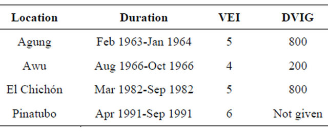
Table 2. Pearson correlation coefficients for 12-month running means of SOI and MGT using different time lags from 1950 to the specified end year (2012 data ends in June) with maximum correlations highlighted for each period.
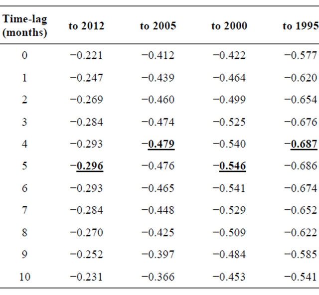
lations occur with a 4-month delay. It is noticeable that correlations deteriorate as the data extend further into the post-2000 period.
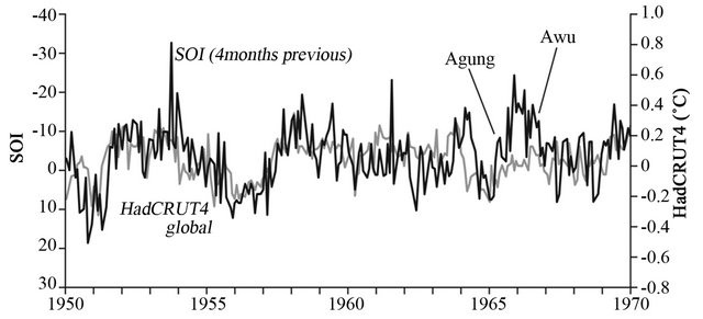
To examine the relationship between the SOI and MGT over the study period, monthly data were plotted together. Figure 1 shows relationship when a 4-month delay is introduced. It shows SOI and MGT cohere over the 62-year period, although the relationship breaks down at times of major volcanic eruptions. Figure 1(c) also shows a clear shift in the lines beginning in the mid- 1990s. This shift is also seen in Figure 2, which shows the difference between mean monthly Northern Hemisphere (NH) temperature anomalies and the mean monthly temperature anomalies for the Southern Hemisphere (SH), that is NH - SH. Because the MGT is (NH + SH)/2, the divergence of NH and SH anomalies naturally causes a shift in the MGT. The reason for this separation beginning in the mid-1990s is not clear.
Figure 3 shows the four-month shifted SOI anomalies alongside monthly MGT anomalies for the period from the beginning of the shift in 1995 to 2012. The dark line indicates SOI and the light line indicates MGT. Note that the Y-axis scale is different to that in Figure 1. It is clear from Figure 3 that the close correlation of MGT and SOI continues after about 1995, albeit with shifted monthly values relative to the earlier data.
4. Discussion and Conclusions
The results show that, by and large, the Southern Oscillation has a consistent influence on mean global temperature. Changes in temperature are consistent with changes in the SOI that occur about four months earlier. The relationship weakens or breaks down at times of major volcanic eruptions. Since the mid-1990s, little volcanic activity has been observed in the tropics and global average temperatures have risen and fallen in close accord with the SOI of four months earlier; although with the unexplained divergence of NH and SH average temperature anomalies modifying the earlier relationship.
The strength of the SOI-MGT relationship may be indicative of the increased vigor in the meridional dispersal of heat during El Niño conditions and the delay in the temperature response is consistent with the transfer of tropical heat polewards. The mechanism of heat transfer is likely the more vigorous Hadley Cell Circulation on both sides of the Intertropical Convergence Zone distributing warm air from the tropical regions to higher latitudes. The process of meridional heat dispersal weakens during La Niña conditions and is accompanied by a lower than normal MGT. Hadley Cell Circulation is weakened when the Southern Oscillation is in a state
 (a)
(a)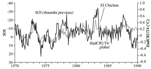 (b)
(b)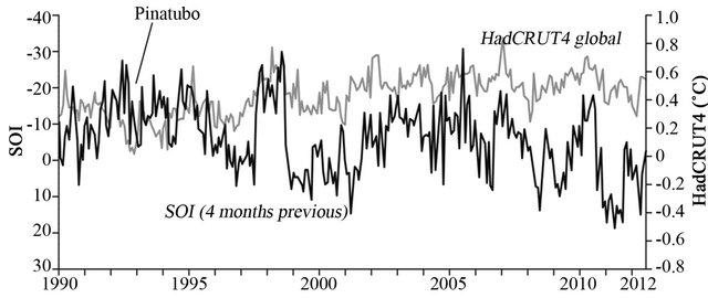 (c)
(c)
Figure 1. Four-month shifted SOI anomalies with monthly MGT anomalies shown for periods 1950 to 1970 (a), 1970 to 1990 (b) and 1990 to June 2012 (c), where the Y-axis scale is identical in each case. The dark line indicates SOI and light line indicates MGT. Periods of volcanic activity are indicated (see text).
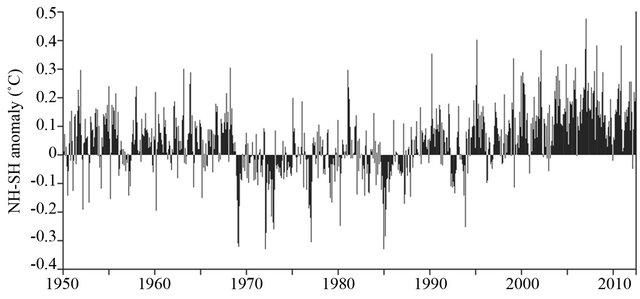
Figure 2. Difference between mean monthly temperature anomalies for the Northern Hemisphere (NH) and Southern Hemisphere (SH).
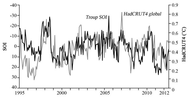
Figure 3. Four-month shifted SOI anomalies with monthly MGT anomalies shown for the period 1995 to June 2012. Dark line indicates SOI and light line indicates MGT. Note the Y-axis scale is different to that in Figure 1.
associated with La Niña conditions (i.e. positive Troup SOI values), but strengthens as the Southern Oscillation moves to a condition consistent with El Niño conditions (that is negative SOI values) [6,7].
The precision of the 4-month lag period is uncertain, but the credibility of a lag of some length is not in dispute. Researchers [31] found that mean tropical temperatures for a 13-year record lagged outgoing longwave anomalies by about three months, while [32] found warming events peak three months after sea surface temperature (SST) in the Niño-3.4 region. On the same theme, [33] founds lags between 1 - 3 months with SST in the Niño-3.4 region for the period 1950-1999. Along the same lines [14] determined that the correlation between SST in the Niño-3 region and the MGT anomaly was optimum with a time lag of 3 - 6 months. The sequence of the lagged relationship indicates that ENSO is driving temperature rather than the reverse. Reliable ENSO prediction is possible only to about 12 months [34], which implies that improved temperature forecasting beyond that period is dependent on advancements in ENSO prediction.
The reason for the post-1995 period shift in the SOIMGT relationship illustrated in Figure 1(c) is puzzling. An explanation may lie in changes in global albedo due to changes in lower-level cloud cover. In an analysis of Australian data, [34] found positive values of SOI anomalies to be associated with increased cloudiness and decreased incoming solar radiation. Data from the International Satellite Cloud Climatology Project (ISCCP) indicate that, from 1984 to 2005, mid-level cloud cover in the tropics was relatively constant but both lower and upper level cloud cover declined slightly. In the exotropics (latitude > 20 degrees, low-level cloud progressively decreased from 1998 onwards. It is not clear whether the change is a cause or an effect of a parallel temperature change [35]. The post-1995 shift appears unrelated to carbon dioxide increase because it occurred long after atmospheric CO2 was known to be rising. It is important to see the shift as more of discrete (i.e. step) change rather than a divergence, with the relationship re-established after 2 - 3 years. Another possibility is that there are problems with the HadCRUT4 1.1.0 data. For example, we note that the published monthly average global temperature anomalies are not equal to the mean of the two published corresponding hemispheric values.
The approach used here avoids a focused statistical analysis of the data, in part because the study deals with smoothed data, which means there is the danger of spurious correlations, and in part because the ENSO is a cyclical phenomenon of irregular period. In these situations, the results of regression analysis or similar statistical evaluation can be misleading. With the potential controversy arising over a particular statistical analysis removed, the findings reported here indicate that atmospheric processes that are part of the ENSO cycle are collectively a major driver of temperature anomalies on a global scale. All other things being equal, a period dominated by a high frequency of El Niño-like conditions will result in global warming, whereas a period dominated by a high frequency of La Niña-like conditions will result in global cooling. Overall, the results imply that natural climate forcing associated with ENSO is a major contributor to temperature variability and perhaps a major control knob governing Earth’s temperature.
REFERENCES
- R. J. Allan, “El Niño Southern Oscillation Influences in the Australasian Region,” Progress in Physical Geography, Vol. 12, No. 3, 1988, pp. 4-40. doi:10.1177/030913338801200301
- R. J. Allan, J. Lindesay and D. Parker, “El Niño Southern Oscillation and Climatic Variability,” CSIRO Publishing, Collingwood, 1996.
- K. E. Trenberth and J. M. Caron, “Estimates of Meridional Atmosphere and Ocean Heat Transports,” Journal of Climate, Vol. 14, No. 16, 2001, pp. 3433-344. doi:10.1175/1520-0442(2001)014<3433:EOMAAO>2.0.CO;2
- K. E. Trenberth, J. M. Caron, D. P. Stepaniak and S. Worley, “Evolution of El Niño-Southern Oscillation and Global Atmospheric Surface Temperatures,” Journal of Geophysical Research, Vol. 107. No. D8, 2002, pp. AAC 5-1-AAC5-17. doi:10.1029/2000JD000298
- N. C. Fernandez, et al., “Analysis of the ENSO Signal in Tropospheric and Stratospheric Temperatures observed by MSU, 1979-2000,” Journal of Climate, Vol. 17, No. 20, 2004, pp. 3934-3946. doi:10.1175/1520-0442(2004)017<3934:AOTESI>2.0.CO;2
- B. Bhaskaran and A. B. Mullan, “El Niño-Related Variations in the Southern Pacific Atmospheric Circulation: Model versus Observations,” Climate Dynamics, Vol. 20, No. 2-3, 2003, p. 229-239.
- A. H. Oort and J. J. Yienger, “Observed Interannual Variability in the Hadley Circulation and Its Connection to ENSO,” Journal of Climate, Vol. 9, No. 11, 1996, pp. 2751-2767. doi:10.1175/1520-0442(1996)009<2751:OIVITH>2.0.CO;2
- M. Indeje, H. M. Semazzi and L. J. Ogallo, “ENSO Signals in East African Rainfall Seasons,” International Journal of Climatology, Vol. 20, No. 1, 2000, pp. 19-46. doi:10.1002/(SICI)1097-0088(200001)20:1<19::AID-JOC449>3.0.CO;2-0
- S. Janicot, S. Trzaska and I. Poccard, “Summer SahelENSO Teleconnections and Decadal Time Scale SST Variations,” Climate Dynamics, Vol. 18, No. 3-4, 2001, pp. 3003-320. doi:10.1007/s003820100172
- H. K. Ntale and T. Y. Gan, “East African Rainfall Anomaly Patterns in Association with El Niño/Southern Oscillation,” Journal of Hydrologic Engineering, Vol. 9. No. 4, 2004, pp. 257-268. doi:10.1061/(ASCE)1084-0699(2004)9:4(257)
- A. Giannini, J. C. H. Chiang, M. A. Cane, Y. Kushnir and R. Seager, “The ENSO Teleconnection to the Tropical Atlantic Ocean: Contributions of the Remote and Local SSTs to Rainfall Variability in the Tropical Americas,” Journal of Climate, Vol. 14, No. 24, 2001, pp. 4530‑4544. doi:10.1175/1520-0442(2001)014<4530:TETTTT>2.0.CO;2
- A. B. Mullan, “Effects of ENSO on New Zealand and the South Pacific,” In D. Braddock, Ed., Prospects and Needs for Climate Forecasting, The Royal Society of New Zealand, Wellington, 1996.
- P. J. Michaels and P. C. Knappenberger, “Natural Signals in the MSU Lower Tropospheric Temperature Record,” Geophysical Research Letters, Vol. 27. No. 18, 2000, pp. 2905-2908. doi:10.1029/2000GL011833
- A. H. Sobel, I. M. Held and C. S. Bretherton, “The ENSO Signal in Tropical Tropospheric Temperature,” Journal of Climate, Vol. 15, No. 18, 2002, pp. 2702-2706. doi:10.1175/1520-0442(2002)015<2702:TESITT>2.0.CO;2
- J. D. McLean, C. R. de Freitas and R. M. Carter, “Influence of the Southern Oscillation on Tropospheric Temperature,” Journal of Geophysical Research, Vol. 114, No. D14, 2009. doi:10.1029/2008JD011637
- T. P. Barnett, “Variations in Near-Global Sea Level Pressure,” Journal of the Atmospheric Sciences, Vol. 42, No. 5, 1985, pp. 478-501. doi:10.1175/1520-0469(1985)042<0478:VINGSL>2.0.CO;2
- C. F. Ropelewski and P. D. Jones, “An Extension of the Tahiti-Darwin Southern Oscillation Index,” Monthly Weather Review, Vol. 115, No. 10, 1987, pp. 2161-2165.
- R. J. Allan, N. Nicholls, P. D. Jones and I. J. Butterworth, “A Further Extension of the Tahiti-Darwin SOI, Early ENSO Events, and Darwin Pressure,” Journal of Climate, Vol. 4, No. 7, 1991, pp. 743-749. doi:10.1175/1520-0442(1991)004<0743:AFEOTT>2.0.CO;2
- Australian Government Bureau of Meteorology, “S.O.I. (Southern Oscillation Index) Archives-1876 to Present,” 29 October 2012. http://www.bom.gov.au/climate/current/soihtm1.shtml
- A. J. Troup, “The Southern Oscillation,” Quarterly Journal of the Royal Meteorological Society, Vol. 91, No. 390, 1965, pp. 490-506. doi:10.1002/qj.49709139009
- C. P. Morice, J. J. Kennedy, N. A. Rayner and P. D. Jones, “Quantifying Uncertainties in Global and Regional Temperature Change Using an Ensemble of Observational Estimates: The HadCRUT4 Dataset,” Journal of Geophysical Research: Atmospheres (1984-2012), Vol. 117, No. D8, 2012. doi:10.1029/2011JD017187
- A. Lacis, J. Hansen and M. Sato, “Climate Forcing by Stratospheric Aerosols,” Geophysical Research Letters, Vol. 19, No. 15, 1992, pp. 1607-1610. doi:10.1029/92GL01620
- M. Sato, J. E. Hansen, M. P. McCormick and J. B. Pollack, “Stratospheric Aerosol Optical Depths, 1850-1990,” Journal of Geophysical Research, Vol. 98. No. D12, 1993, pp. 22987-22994.
- C. F. Mass and D. A. Portman, “Major Volcanic Eruptions and Climate: A Critical Evaluation,” Journal of Climate, Vol. 2, No. 6, 1989, pp. 566-593. doi:10.1175/1520-0442(1989)002<0566:MVEACA>2.0.CO;2
- E. G. Dutton and J. R. Christy, “Solar Radiative Forcing at Selected Locations and Evidence for Global Lower Tropospheric Cooling Following the Eruptions of El Chichón and Pinatubo,” Geophysical Research Letters, Vol. 19, No. 23, 1992, pp. 2313-2316. doi:10.1029/92GL02495
- C. G. Newhall and S. Self, “The Volcanic Explosivity Index (VEI): An Estimate of Explosive Magnitude for Historical Volcanism,” Journal of Geophysical Research, Vol. 87. No. C2, 1982, pp. 1231-1238. doi:10.1029/JC087iC02p01231
- H. H. Lamb, “Volcanic Dust in the Atmosphere; With a Chronology and Assessment of Its Meteorological Significance,” Philosophical Transactions of the Royal Society of London, Series A, Vol. 266, No. 1178, 1970, pp. 425-533. doi:10.1098/rsta.1970.0010
- H. H. Lamb, “Supplementary Volcanic Dust Veil Assessments,” Climate Monitor, Vol. 6, 1977, pp. 57-67.
- H. H. Lamb, “Update of the Chronology of Assessment
- of the Volcanic Dust Veil Index,” Climate Monitor, Vol. 12, No. 1178, 1983, pp. 79-90.
- D. Douglass and R. S. Knox, “Climate Forcing by the Volcanic Eruption of Mount Pinatubo,” Geophysical Research Letters, Vol. 32, No. 5, 2005.
- E. Yulaeva and J. M. Wallace, “The Signature of ENSO in Global Temperature and Precipitation Fields Derived from the Microwave Sounding Unit,” Journal of Climate, Vol. 7, No. 11, 1994, pp. 1719-1736. doi:10.1175/1520-0442(1994)007<1719:TSOEIG>2.0.CO;2
- A. Kumar and M. P. Hoerling, “The Nature and Causes for the Delayed Atmospheric Response to El Niño,” Journal of Climate, Vol. 16. No. 9, 2003, pp. 1391-1403. doi:10.1175/1520-0442-16.9.1391
- S. Solomon, D. Qin, M. Manning, Z. Chen, M. Marquis, K. B. Averyt, M. Tignor and H. L. Miller (Eds.), “Climate Change 2007: The Physical Science Basis. Contribution of Working Group I to the Fourth Assessment Report of the Intergovernmental Panel on Climate Change,” Cambridge University Press, Cambridge, 2007, p. 996.
- D. A. Jones and B. C. Trewin, “On the Relationship between the El Nino-Southern Oscillation and Australian Land Surface Temperature,” International Journal of Climatology, Vol. 20, No. 7, 2000, pp. 697-719. doi:10.1002/1097-0088(20000615)20:7<697::AID-JOC499>3.0.CO;2-A
- R. W. Spencer and W. D. Braswell, “Potential Biases in Feedback Diagnosis from Observational Data: A Simple Model Demonstration,” Journal of Climate, Vol. 21, No. 21, 2008, pp. 5624-5628. doi:10.1175/2008JCLI2253.1
NOTES
*Corresponding author.