International Journal of Geosciences
Vol. 4 No. 2 (2013) , Article ID: 28925 , 12 pages DOI:10.4236/ijg.2013.42027
Parameters Identification of Stochastic Nonstationary Process Used in Earthquake Modelling
1Department of Civil and Architectural Science, Technical University of Bari, Bari, Italy
2Mobility Department, AIT Austrian Institute of Technology GmbH, Vienna, Austria
Email: g.c.marano@gmail.com
Received September 8, 2012; revised December 12, 2012; accepted January 17, 2013
Keywords: Seismic Analysis; Random Vibrations; Non-Stationary Process
ABSTRACT
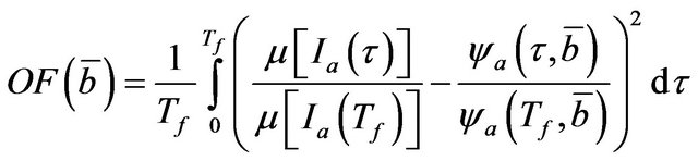
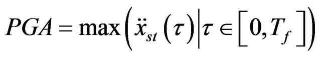
This paper proposes a new deterministic envelope function to define non-stationary stochastic processes modeling seismic ground motion accelerations. The proposed envelope function modulates the amplitude of the time history of a stationary filtered white noise to properly represent the amplitude variations in the time histories of the ground motion accelerations. This function depends on two basic seismological indices: the Peak Ground Acceleration (PGA) and the kind of soil. These indices are widely used in earthquake engineering. Firstly, the envelope function is defined analytically from the Saragoni Hart’s function. Then its parameters are identified for a set of selected real records of earthquake collected in PEER Next Generation Attenuation database. Finally, functions of the parameters depending on the Peak Ground Acceleration and the kind of soil are defined from these identified values of the parameters of the envelope function through a regression analysis.
1. Introduction
The improvement of the accuracy and the robustness of the structural design in seismic areas is the aim of the seismic engineering. In order to define rules in the design codes for structures resistant to seismic loads, several scientists have investigated the probability of occurrence, the intensity and the frequency of a seismic event in a specific area. Indeed, these characteristics of the possible earthquake occurring in an area define the seismic dynamic load that could excite a structure during its lifetime. The structural response depends also on some characteristics of the seismic load related to some seismological parameters, like the event intensity, the rupture type and the epicentral distance. Unfortunately, these seismological parameters are not very useful in structural design. Indeed, the seismic design is based on the knowledge of the characteristics of the seismic ground motions in time domain, as the maximum amplitude, the period and the duration, and in frequency domain, as the Fourier spectrum and the response spectrum. The analysis of the structural response to real occurred seismic events or to synthetic accelerograms related to that seismic area is necessary to design a structure in a seismic area. For this reason several methods have been already proposed to model earthquakes and generate synthetic accelerograms.
Nonlinear time-history procedures are increasingly used for structural and geotechnical analyses [1], but they have not yet been adopted widely because of their higher computational cost in comparison with the equivalent static analyses. Actually this reason is not more tenable because of the increasing power of computers. On the other hand, it is necessary to take into account the difficulty to obtain natural earthquake accelerograms that adhere to some criteria such as the spectrum for some design scenarios. This difficulty is overcome by adopting modified natural records (modified through adjustments either in the time domain or in frequency domain) or synthetic accelerograms in the analyses instead of real records of the ground motion acceleration. The approach based on the natural accelerograms is prevalent, because a real recorded accelerogram properly processed is undeniably a realistic representation of the ground shaking occurring in a specific seismological scenario. On the other hand, a real accelerogram is the record of a past seismic event and it could differ from the future ground motions, while the artificial accelerograms sometimes approximate the future earthquakes very well.
The earthquakes are stochastic events, so in most of the studies each single seismic event is defined as a sample function of a stochastic process that models the earthquake ground motion occurring in a specific area. This stochastic process modelling the earthquake occurring in an area is defined through the characteristics of the strong ground motions recorded in that area. The stochastic-based approach is the most suitable to model earthquake records owing to the complex nature of the release of the seismic waves and their propagation in the soil. The synthetic accelerograms used to predict the maximum response of structures and infrastructures to future earthquakes are estimated as samples of the stochastic process modelling the earthquake in that area.
In the last century several scholars proposed methods to define the stochastic process modelling the earthquake occurring in a specific area. Firstly, the stationary white noise process was used to model the earthquake. Afterwards, in other studies the earthquake was modelled through a stationary filtered white noise process. Among these models based on the stationary filtered white noise there are the Kanai-Tajimi model ([2,3]) and its modifications [4]. Housner and Jennings [5] proposed a method to model the ground motion as a stationary filtered white noise process (according to the Kanai-Tajimi model) by means of parameters used in seismic engineering.
As shown in some studies, the ground motion records are non-stationary. They have variation both in the amplitude and the frequency content through their duration. For this reason some scholars proposed to use a weakly stationary process to model the earthquake ground motion. In these models the component of the process that dominates amplitude-based measures of the structural response is well represented. In order to define the nonstationary stochastic process modelling the earthquake in a given area, several scholars have multiplied a stationary stochastic process by an envelope function (Figure 1), as Bolotin [6]. He has proposed a deterministic envelope function that modulates a White Noise (WN) filtered by a linear Single Degree of Freedom (SDOF) system. Jangid [7] has presented an overview of the envelope functions proposed in literature. These functions have simple parametric forms. They describe the evolution of the ground shaking amplitude during the earthquake and define the strong motion duration. A great deal of efforts has been already focused on the research of a reliable envelope function to model the ground motion intensity. To better tune up the artificial accelerograms to real recorded ones different kind of shaping window were proposed, like trapezoidal, double exponential and log-normal. Some envelope functions proposed in literature correlate the law of the evolution of the ground acceleration amplitude in time domain for seismic events expected in a site with some characteristics of both the site and the earthquakes occurred in that area. The envelope functions proposed in some studies ([8,9]) are correlated with a large number of seismological parameters that are not useful indices in the seismic design, as afore said. Also in the paper [10] seismological data have been used to define the envelope function modulating a stationary stochastic process to generate synthetic accelerograms. Baker [11] has presented a relation among the ground motion intensity parameters used to predict the structural and geotechnical response.
In literature only very few studies have proposed envelope functions related to the characteristics of the ground motions used in the seismic design. The study presented in this article makes an effort in that direction. The simple envelope function proposed here depends on only two characteristics of the seismic ground motion used in the seismic design: the PGA and the soil type. For this reason the function is effective in generating artificial accelerograms useful for the seismic design purposes. The function is deterministic and is based on the Saragoni and Hart’s (SH) exponential model [12] with three parameters determined through an energetic criterion. This kind of envelope function gives the best agreement with selected time-histories, as a numerical analysis shows hereafter. This function is calculated through a procedure composed by two stages. Firstly an analytical envelope function derived from the Saragoni and Hart’s one is defined. This function is called Modified Saragoni and Hart’s (MSH) envelope function. The MSH function is obtained from the analytical relations of the Saragoni and Hart’s function and the Arias Intensity (AI). The parameters of the MSH function are calculated through an identification procedure applied to various sets of accelerograms characterized by different values of PGA and different kind of soil. The identified values of the parameters are the ones that minimize the differences related to the AI of each real accelerogram and the AI of MSH modulation function. Thus, a regression law for each parameter of the MSH function is estimated from the values of the same parameters identified by using the real earthquake records. Therefore, the regression laws result to be function of the kind of soil and the PGA.
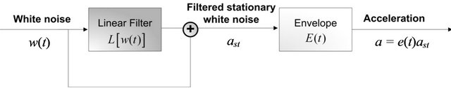
Figure 1. Scheme to generate synthetic accelerograms.
2. Stationary Stochastic Process Modelling the Seismic Ground Motion
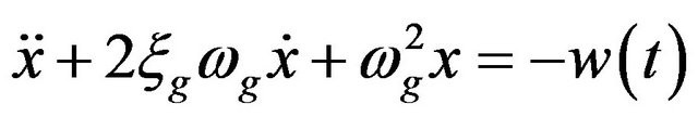
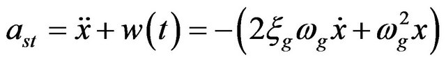
As said in the previous section, a simple model used to represent an earthquake accelerogram is a filtered stationary noise . This signal has the real frequency content of the earthquake acceleration. In this kind of model a WN models the earthquake acceleration at the bedrock, while a SDoF system defines the filtering effects of the soil layer crossed. Indeed the soil filters the frequency content of the signal. Two parameters characterizes this SDoF system: the damping ratio
  and the circular frequency
 . The ground acceleration
  is defined as the absolute acceleration of the filter:
 (1)
(1)
 . (2)
. (2)
The power spectral density function of the filtered WN is
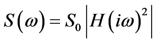 , (3)
, (3)
where 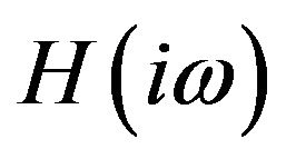 is the complex frequency response function of the filter and
  is the Power Spectral Density (PSD) of the WN excitation. This filter is a linear second order one, so the PSD of the filtered process is
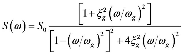 . (4)
. (4)
This model to estimate the PSD of the earthquake acceleration is known as the Kanai-Tajimi one ([2,3] and [13]). The Kanai-Tajimi model does not represent well the earthquake ground motion characterized by medium and long period, because only two filter parameters (the damping ratio and the circular frequency of the filter) describe it. In order to overcome this limit, Clough and Penzien [14] proposed a model characterized by a linear double filter forced by a WN. In this model the ground acceleration  is given by:
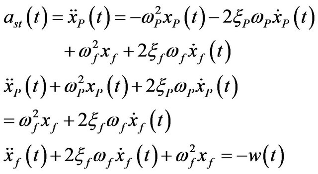 (5)
(5)
where  is the response of the first filter characterized by the circular frequency
  and the damping ratio
 ,
,  is the response of the second filter characterized by the circular frequency
  and the damping ratio
  and
and  is the WN process. In this model the stationary ground acceleration coincides with the acceleration of the second filter output
 .
.
More complex methods were proposed to calculate the seismic ground acceleration. Some researchers ([15,16]) have taken into account the non-stationarity of the earthquake ground motion in time domain and proposed methods to model it as a weakly non-stationary stochastic process. Other scholars have modelled the earthquake as a non-stationary stochastic process to consider the nonstationarity both in time and frequency domain [16]. Indeed, the earthquake ground motion is non-stationary in the time domain due to the temporal variation of the ground acceleration intensity and in frequency domain owing to the temporal variation of the frequency content evaluated in each earthquake record of a specific area.
In literature other more complex approaches characterized by Multi Degree of Freedom (MDoF) filters have been proposed to simulate the shear wave of earthquake events: these models are described by a larger number of parameters than the KT and CP models parameters, so they model the soil filtering effect of the seismic waves in better way than the KT and CP models, but they require a higher computational effort.
The Clough-Penzien model could be used to define the frequency content of the seismic ground motion, while the amplitude modulation in time could be modelled by the envelope function proposed here.
3. Definition of the Envelope Function
In several previous studies and in this paper the nonstationary stochastic process modelling the seismic ground motion is obtained by multiplying a simulated stationary process  by an envelope function
 :
:
 . (6)
. (6)
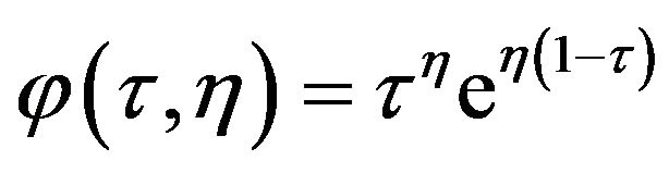
A new envelope function is proposed in this paper. It is obtained from a complex procedure described hereafter. Firstly, a function that approximates the real envelope of selected recorded accelerograms is estimated and it is called pre-envelope functions. Its shape is similar to the envelope function proposed by Saragoni and Hart [12]. This envelope function is exponential and deterministic. It is selected here among the other modulation functions because the arbitrary division into segments and the abrupt change in the frequency content of each segment peculiar to most of the other modulation function are not very satisfactory to simulate strong ground motion. The Saragoni and Hart’s (SH) function has the following shape:
 , (7)
, (7)
where ,
,  and
and  are the calibration parameters. In the first part of the procedure to define the envelope function the parameters of the function are identified from a large set of real accelerograms. To perform the identification procedure, the two parameters
  and
and  are expressed as functions of the unknown time
  in which the modulation function presents its maximum value. The maximum value of the modulation function is estimated by solving the system of equations:
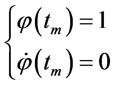 (8)
(8)
The two parameters  and
and  are evaluated from the Equation (8) as function of the other two parameters
  and
and :
:
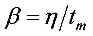 , (9)
, (9)
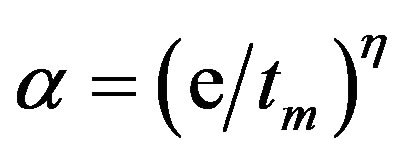 . (10)
Using the Equations (9) and (10), the SH function (Equation (7)) can be written as function of only the two parameters  and
and  that define the shape of envelope:
 , (11)
where . The real seismic events are not well described by only their peak values, such as PGA, but also by the energy content and the quantities related to it, such as the Arias Intensity (AI). The expression of the AI is
 . (12)
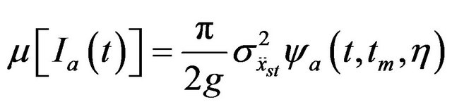
The mean value of the AI in stochastic terms is
 (13)
(13)
where  is the total duration time of the earthquake,
  is the ground acceleration at time
  in one of the two horizontal directions,
  is gravity acceleration and
  is defined by the expression
 . (14)
Now introducing the envelope function (11) in the Equation (14) it becomes
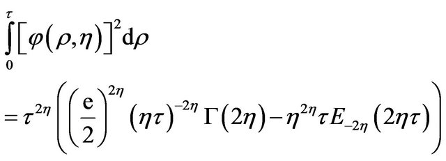 (15)
(15)
where 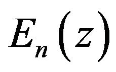 is the generalized exponential integral function
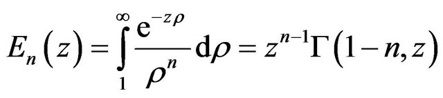 (16)
(16)
while  is the Euler Gamma function
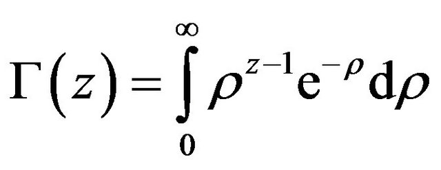 (17)
(17)
In the Figure 2 the dimensionless ratio 
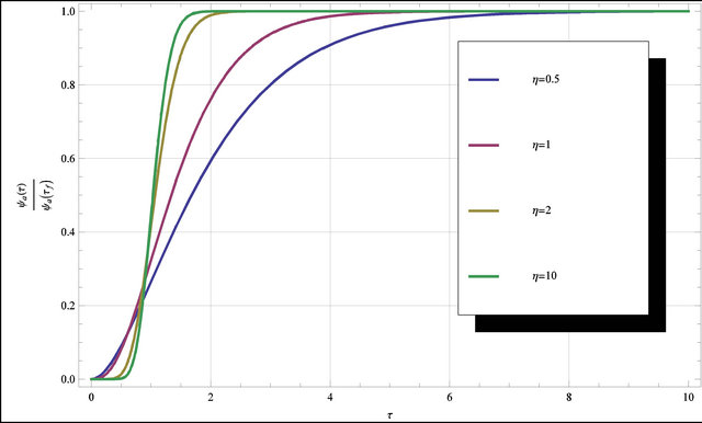
Figure 2. Sensitivity of the term  of the envelope function related to the energy release to the parameter
 .
.
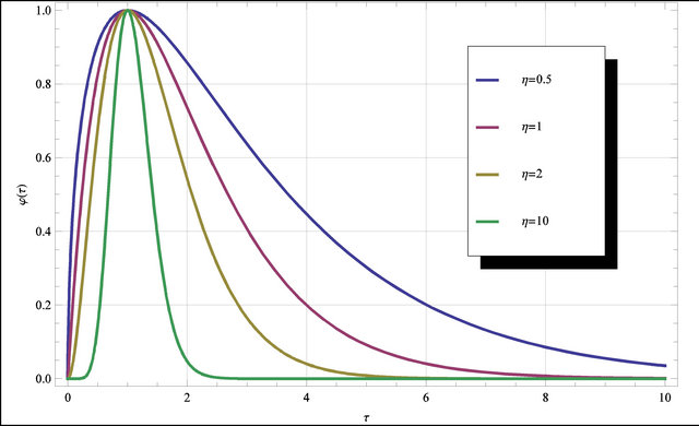
Figure 3. Sensitivity of the term  of the envelope function to the parameter
 .
.
is plotted for different values of the parameter . This ratio is a function only of the parameters
  and
and  that describe the intensity modulation in time of the earthquake acceleration. From that figure it is clear that the energy release is strongly influenced by the parameter
 : the total energy is related to different time ratio
  for each value of the parameter
 . In the Figure 3 the value of the parameter
  is plotted against the value of the parameter
  for different value of
 .
.
4. Numerical Procedure to Evaluate the Process Parameters
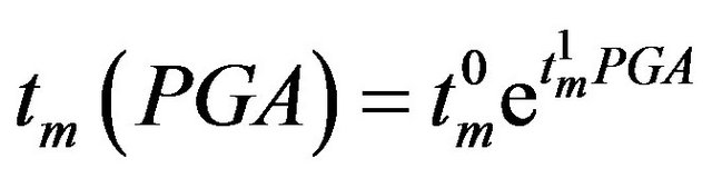
This section describes the procedure to calculate the values of the parameters  and
and  that fit each of the selected real accelerograms of the PEER Next Generation Attenuation database. These parameters describe the preenvelope function of the selected real accelerograms of the PEER Next Generation Attenuation database.
The selected records of the PEER Next Generation Attenuation database match the following criterion: the sites where the accelerograms were recorded have an average shear wave velocity in the top 30 m comprised in four ranges according to the EC8 and the NERPH classification. The ground motion records of the PEER Next Generation Attenuation ground motion database are more than 7000 and half of them matches this criterion. Moreover, the ground acceleration records of both the horizontal directions are used to estimate a mean value of each seismic event: the weighted square root of the sum of the squares of the east-west and north-south components is calculated. This weighted mean value is used to estimate the pre-envelope mean function and the PGA for each seismic event.
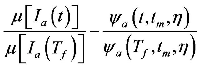
The value of the modulation function parameters for each seismic event are obtained by minimizing the difference between two ratios: the ratio of the mean values of the AI for the real earthquake record that describes the progressive energy release during the duration of that earthquake and the ratio of parameter related to the energy release in the mean value of the AI of the accelerogram modulated by the MSH function
 . (18)
The ratios of the Equation (18) measure the progresssive energy release during the earthquake as function of the total duration  of the seismic event. This duration is defined as the time during which the 98% of the total seismic signal energy is released. This time is evaluated as the time window that elapses from 1% to 99 % of the AI of the given seismic signal. The total duration is calculated for each selected weighted accelerogram of the database. The total duration and the Equation (18) define the Objective Function (OF) of the optimization problem solved to estimate the couple of parameters
  and
and  for each weighted accelerogram selected from the database:
 (19)
(19)
where 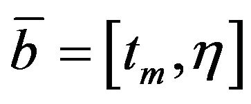 is the variable vector. The optimization problem is solved by using the Genetic Algorithm (GA) implemented in Matlab. The results of the identification procedures applied to a real earthquake record are shown in the Figures 4 and 5.
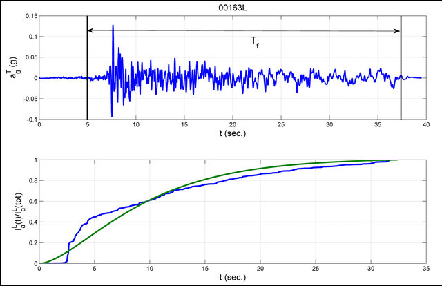
Figure 4. The record 00163 of the database in longitudinal direction (L) and its total duration time are shown. Ratio of the progressive Arias Intensity and the total Arias Intensity estimated for the record 00163L. The blue line indicates the value for the real record and the green line indicates the analytical value.
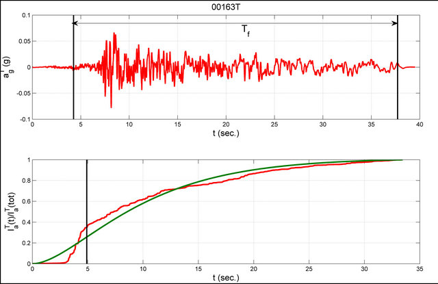
Figure 5. The record 00163 of the database in transversal direction (T) and its total duration time are shown. Ratio of the progressive Arias Intensity and the total Arias Intensity estimated for the record 00163T. The red line indicates the value for the real record and the green line indicates the analytical value.
Each identified couple of parameters  and
and  describes the pre-envelope function of the respective real seismic event selected from the database. The selected earthquakes records of the PEER Next Generation Attenuation database and consequently the identified parameters are grouped according to the four types of soil defined in EC8 and NERPH, so the couples of identified parameters describe the pre-envelope functions (MSH functions) for each earthquake record selected from the database. After the identification of the parameters couples the mean value of analytical expression of the AI is calculated. Using the values of the parameters
  and
and  computed by means of the identification procedure:
 . (20)
Then a linear function is used to correlate the maximum peak of the ground acceleration with its stationary variance 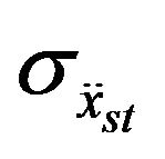 at the time
 :
:
 , (21)
where
 . (22)
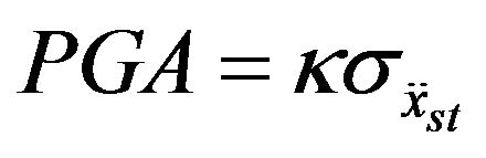
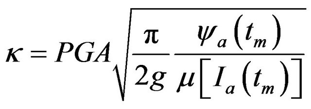
The definition of the PGA is
 (23)
(23)
where  is again the total duration of the earthquake, then
 . (24)
From the evaluation of (2) it is possible also calculate a new intensity measure  called Envelope Intensity (EI) and defined as:
 . (25)
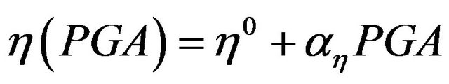
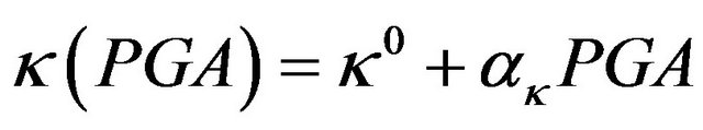
5. Regression Laws
In the second stage of the procedure the regression laws of same parameters (the total duration time , the AI
 , the maximum envelope time
 ,
,  and
and ) of the MSH function are estimated from the pre-envelope functions. These regression laws relate the parameters of the envelope function to the PGA. The functions obtained from the regression analysis of the values of the pre-envelope functions are:
 , (26)
 , (27)
 , (28)
 , (29)
 , (30)
where the PGA is express in g (9.81 m/sec2). The Figures 6-9 show the values of the parameters  and
and  for the pre-envelope functions of the set of seismic events selected from the database. In these figures also the regression laws for these parameters are plotted with red lines. The Figures 10-13 show the values of the
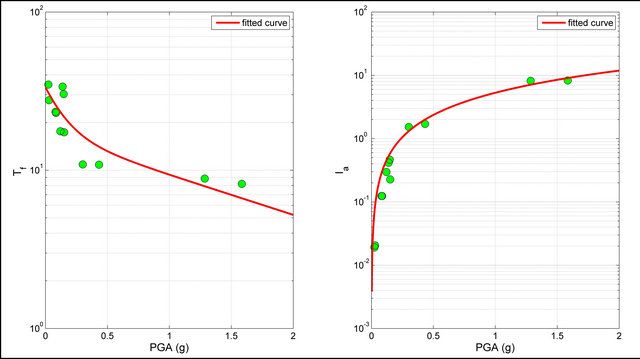
Figure 6. Values of  and
and  defined as function of the PGA. The values are related to the set of the seismic events selected from the database and occurred in sites characterized by kind of soil A.
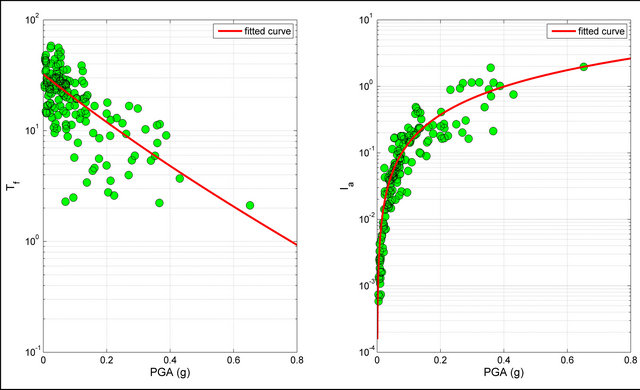
Figure 7. Values of 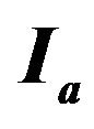 and
and  defined as function of the PGA. The value are related to the set of the seismic events selected from the database and occurred in sites characterized by kind of soil B.
Figure 8. Values of  and
and  defined as function of the PGA. The value are related to the set of the seismic events selected from the database and occurred in sites characterized by kind of soil C.
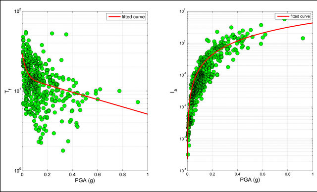
Figure 9. Values of  and
and  defined as function of the PGA. The value are related to the set of the seismic events selected from the database and occurred in sites characterized by kind of soil D.
Figure 10. Values of ,
,  and
and  defined as function of the PGA. The value are related to the set of the seismic events selected from the database and occurred in sites characterized by kind of soil A.
Figure 11. Values of ,
,  and
and  defined as function of the PGA. The value are related to the set of the seismic events selected from the database and occurred in sites characterized by kind of soil B.
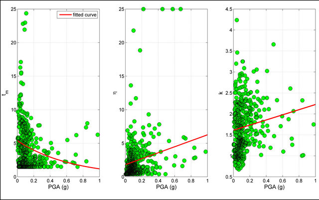
Figure 12. Values of ,
,  and
and  defined as function of the PGA. The value are related to the set of the seismic events selected from the database and occurred in sites characterized by kind of soil C.
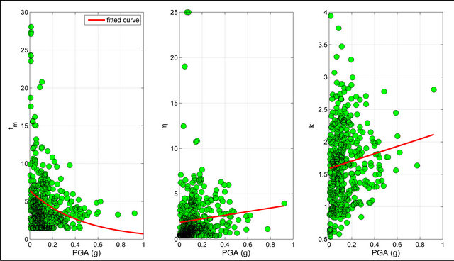
Figure 13. Values of ,
,  and
and  defined as function of the PGA. The value are related to the set of the seismic events selected from the database and occurred in sites characterized by kind of soil D.
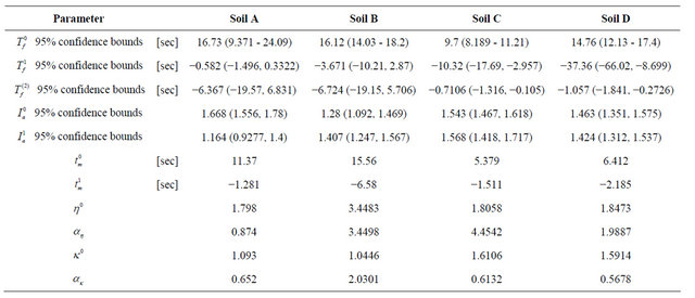
Table 1. Values of the parameters estimated with the regression analysis grouped the kind of soil.
parameters ,
,  and
and  for the pre-envelope functions of the set of seismic event selected from the database. In these figures also the regression laws for these parameters are plotted with red lines.
6. Results Analysis and Conclusions
In the Figures 6-9 the regression law of the AI (Equation (27)) matches perfectly the trend of the AI valuated from the real data, while the curves of the regression law for the other parameters do not tally with the values estimated from the real earthquake records selected from the database.
The main purpose of the proposed procedure is to obtain the mean values of the parameters estimated through the identification procedure applied to a given set of real earthquake grouped according to the kind of soil.
The mean values obtained through the regression analysis have been collected in Table 1 and they could be used in the MSH envelope function to modulate the amplitude of synthetic accelerograms.
REFERENCES
- K. Beyer and J. J. Bommer, “Selection and Scaling of Real Accelerograms for Bi-Directional Loading: A Review of Current Practice and Code Provisions,” Journal of Earthquake Engineering, Vol. 11, No. S1, 2007, pp. 13-45. doi:10.1080/13632460701280013
- K. Kanai, “Semi-Empirical Formula for the Seismic Characteristics of the Ground Motion,” Bulletin of the Earthquake Research Institute, Vol. 35, No. 2, 1957, pp. 309- 325.
- H. Tajimi, “A Statistical Method of Determining the Maximum Response of a Building Structure during an Earthquake,” Proceedings of the 2nd World Conference on Earthquake Engineering, Tokio, 11-18 July 1960, pp. 781-798.
- S. Sgobba, G. C. Marano, P. J. Stafford and R. Greco, “Seismologically Consistent Stochastic Spectra,” New Trends in Seismic Design of Structures, Saxe-Coburg Publisher, Stirling, 2009.
- G. W. Housner and P. C. Jennings, “Generation of Artificial Earthquakes,” ASCE, Journal of the Engineering Mechanics Division, Vol. 90, No. 1, 1964, pp. 113-150.
- V. V. Bolotin, “Statistical Theory of the Aseismic Design of Structures,” Proceedings of the 2nd World Conference on Earthquake Engineering, Tokio, 11-18 July 1960, pp. 1365-1374.
- R. S. Jangid, “Response of SDOF System to Non-Stationary Earthquake Excitation,” Earthquake Engineering & Structural Dynamics, Vol. 33, No. 15, 2004, pp. 1417- 1428. doi:10.1002/eqe.409
- K. W. Campbell, “Prediction of Strong Ground Motion Using the Hybrid Empirical Method: Example Application to Eastern North America,” Bulletin of the Seismological Society of America, Vol. 93, No. 3, 2002, pp. 1012-1033. doi:10.1785/0120020002
- G. Cua, “Creating the Virtual Seismologist: Developments in Ground Motion Characterization and Seismic Early Warning,” Ph.D. Thesis, California Institute of Technology, 2005.
- P. J. Stafford, S. Sgobba and G. C. Marano, “An EnergyBased Envelope Function for the Stochastic Simulation of Earthquake Accelerograms,” Soil Dynamics and Earthquake Engineering, Vol. 29, No. 7, 2009, pp.1123-1133. doi:10.1016/j.soildyn.2009.01.003
- J. W. Baker, “Correlation of Ground Motion Intensity Parameters Used for Predicting Structural and Geotechnical Response,” Proceedings of the 10th International Conference on Applications of Statistics and Probability in Civil Engineering, Tokyo, 31 July- 3 August 2007.
- G. R. Saragoni and G. C. Hart, “Simulation of Artificial Earthquake,” Earthquake Engineering and Structural Dynamics, Vol. 2, No. 3, 1974, pp. 249-267. doi:10.1002/eqe.4290020305
- G. C. Marano, M. Morga and S. Sgobba, “Modelling of Stochastic Process for Earthquake Representation as Alternative Way for Structural Seismic Analysis: Past, Present and Future,” International Conference on Earthquake Analysis and Design of Structures, 1-3 December 2011, Coimbatore, pp. 61-73.
- R. W. Clough and J. Penzien, “Dynamics of Structures,” McGraw-Hill, New York, 1975.
- M. Amin and A. H. S. Ang, “Nonstationary Stochastic Model of Earthquake Motions,” ASCE, Journal of the Engineering Mechanics Division, Vol. 94, No. 2, 1968, pp. 559-583.
- J. P. Conte and B. F. Peng, “Fully Nonstationary Analytical Earthquake Ground-Motion Model,” ASCE, Journal of Engineering Mechanics, Vol. 12, No. 1, 1997, pp. 15-24. doi:10.1061/(ASCE)0733-9399(1997)123:1(15)