Open Journal of Optimization
Vol. 2 No. 2 (2013) , Article ID: 33235 , 7 pages DOI:10.4236/ojop.2013.22007
Optimization Scheme Based on Differential Equation Model for Animal Swarming
Department of Information and Physical Sciences, Osaka University, Osaka, Japan
Email: atsushi-yagi@ist.osaka-u.ac.jp
Copyright © 2013 Takeshi Uchitane, Atsushi Yagi. This is an open access article distributed under the Creative Commons Attribution License, which permits unrestricted use, distribution, and reproduction in any medium, provided the original work is properly cited.
Received March 21, 2013; revised May 6, 2013; accepted May 21, 2013
Keywords: Optimization Scheme; Differential Equation Model; Animal Swarming
ABSTRACT
This paper is devoted to introducing an optimization algorithm which is devised on a basis of ordinary differential equation model describing the process of animal swarming. By several numerical simulations, the nature of the optimization algorithm is clarified. Especially, if parameters included in the algorithm are suitably set, our scheme can show very good performance even in higher dimensional problems.
1. Introduction
Let  be a real valued continuous function defined for
 , where
  is a positive integer. The problem of finding the minimal value
is called a D-dimensional optimization problem for . Such an optimization problem is one of fundamental problems in the study of science and technology and so far various methods have already been presented.
When  is a
is a  function, the point
 ![]() which hits the minimal value
which hits the minimal value  is obtained in the set of solutions of the functional equation
 . But, in general, it is not so easy to solve this functional equation. So, approximate solutions become more important. The steepest descent method is a method of obtaining a sequence
  in
in  which approaches to
 ![]() by using the recurrence formula
by using the recurrence formula
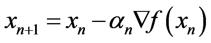 with some suitable coefficient
 . This method is very convenient and it is easily observed that
  converges to a limit
  such that
 . But
. But  may hit very often some local minimal value of
  and not the very minimal value. So, when
  possesses many local minimal values, it is very difficult to find out the point
 ![]() by this method.
by this method.
Recently, a development of techniques of numerical computations has yielded a new paradigm of optimization using a collection of particles in  which interact each other and move for striking out the point
![]() . Such a method is called the particle optimization. One of the typical particle optimization was devised by KennedyEberhart [1]. They consider a swarm of particles not only flying in
. Such a method is called the particle optimization. One of the typical particle optimization was devised by KennedyEberhart [1]. They consider a swarm of particles not only flying in  like bird but also behaving as an intellectual individual which can memorize its personal best through the whole past and, on the other hand, can know the swarm’s global best at each instant. In each step, processing such personal and swarm information, they move to a suitable position. The phase space in which the particles move about is therefore an abstract multi-dimensional space which is collision-free. They called their method the particle swarm optimization. Afterword, the particle swarm optimization has been developed extensively and applied to various problems. We will here quote only some of them [2-4]. A survey of the method has recently been published by Eslami-Shareef-Khajehzadeh-Mohamed [5].
In this paper, we want to compose another type particle optimization which is inspired more directly from the animal swarming like fish schooling, bird flocking, or mammal herding. Our particles move truly according to the animal’s behavioral rules for forming swarm. We first set a D-dimensional physical space  in which the particles move about. We then assume among individuals two kinds of interactions, attraction and collision avoidance. These interactions will be formulated by generalized gravitation laws. Regarding
  as an environmental potential, we assume also that the particles are sensitive to the gradient of
  at their positions and have tendency to move toward the most descending direction of the value of
 . But they cannot know which mate has the global best position of the swarm at any momemt. We will also incorporate uncertainty of their information processing and executing. The phase space of particles is therefore given by
 , here
  means that at that moment the i-th particle is at position xi with velocity vi. As for animal’s behavioral rules, we are going to follow those presented by Camazine-Deneubourg-Franks-Sneyd-Theraulaz-Bonabeau ([6], Chapter 11). That is:
1) The swarm has no leaders and each individual follows the same behavioral rules;
2) To decide where to move, each individual uses some form of weighted average of the position and orientation of its nearest neighbors;
3) There is a degree of uncertainty in the individual’s behavior that reflects both the imperfect informationgathering ability of an animal and the imperfect execution of its actions.
(We refer also a similar idea due to Reynolds [7].) The authors have in facttried to model in the previous paper [8] these mechanisms by stochastic differential Equations (2.1) and (2.2) below.
Our optimization scheme is actually composed on the basis of the continuous model Equations (2.1), (2.2) but just ignoring velocity matching (i.e., taking ) and setting the external force as the sum of resistance and gradient of the potential function to be optimized. At each step, the particles have a velocity determined by the sum of centering with nearby mates and acceleration by the external force. Its position is renewed by the sum of the velocity and a noise which reflects the imperfectness of information-gathering and execution of actions. At the first stage, the particles move striking out the global minimal value on one hand keeping a swarm and on the other hand keeping a territorial distance with other mates. The noise helps the swarm to escape from the traps of local minimal values and to reach into a neighborhood of the global one. At the second stage, the movement of particles slows down. The particles go to an equilibrium state in which some particle attains at the swarm’s best value.
In order to investigate swarm behavior of particles, we shall apply our optimization scheme to a few benchmark problems. When  has many local minimal values, the territorial distance must be chosen in a suitable length to find a good approximate solution. Optimal strength of noise is also required. If it is too small, the swarm is easily trapped by a local minimum; to the contrary, if too large, the particles cannot keep on swarming because of the strong dispersion. If these are suitably set, then our scheme can show very high performance even in 12- dimensional problems.
2. Continuous Model
We being with reviewing the continuous model presented by [8].
We consider motion of I animals in the physical space . The position of i-th animal is denoted by
 , and its velocity by
 . The model equations are then written as
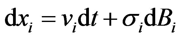 (2.1)
(2.1)
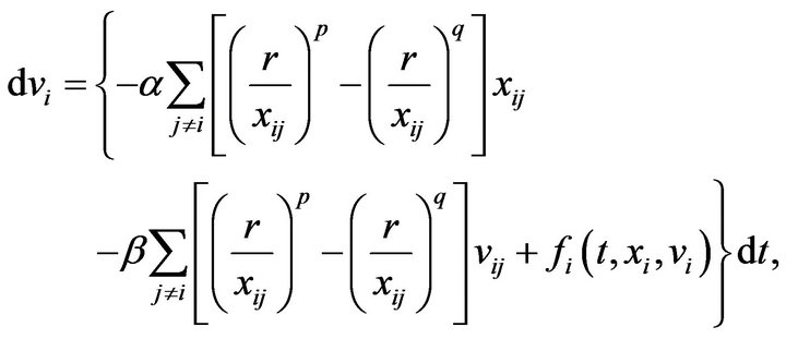 (2.2)
(2.2)
where 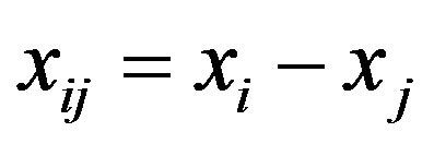 and
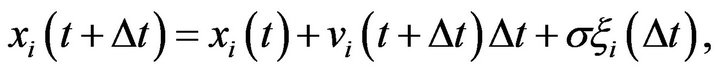
and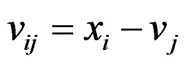 . The first Equation (2.1) is a stochastic equation for xi, here
 denotes a system of independent 3-dimensional Brownian motions defined on a complete probability space with filtration
  (see [9]). The term
  therefore denotes a noise resulting from the imperfectness of information-gathering and action of the i-th animal,
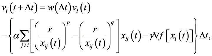
  being some coefficient. In the meantime, (2.2) is a deterministic equation for vi. The first term in the right hand side denotes the centering and the collision avoidance of animal. The animals have tendency to stay nearby their mates and at the same time avoid colliding each other. As p and q are such that
 , if
, if , then the
  -th animal moves toward the j-th; to the contrary, if
 , then it acts in order to avoid collision with the other. The number
  therefore denotes a critical distance. If p is large, then, as the distance
  increases, its power
  decreases quickly. Hence, the larger p is, the shorter the range of centering is. The second term of (2.2) denotes the effect of velocity matching with nearby mates. Finally, the term
  denotes an external force imposed to the i-th animal at time t which is a given function for xi and vi. In the subsequent section, we take a function of the form
 (2.3)
(2.3)
where  denotes a resistance for motion and
  denotes an external force determined by a
  potential function
 .
.
3. Optimization Scheme
Let  be a real valued
  function defined for
  with positive integer
 . Consider the optimization problem
 (3.1)
(3.1)
On the basis of (2.1), (2.2), we introduce an optimization algorithm for (3.1). Let , denote the positions of I particles moving about in the space
 , and let
 , denote their velocities. We ignore velocity matching of particles, namely, we set
 , and take the function
  in (2.2) in the form (2.3) above. Our scheme is then described by
 (3.2)
(3.2)
 (3.3)
(3.3)
where . In addition,
 , is a family of independent stochastic functions defined on a complete probability space
  with values in
  whose distributions are a normal distribution with mean 0 and variance
 . And
. And  is given by
 .
.
Set initial positions and initial velocities
respectively. Then, the algorithm (3.2), (3.3) defines a discrete trajectory
where . In each step n, we compute the minimal value
 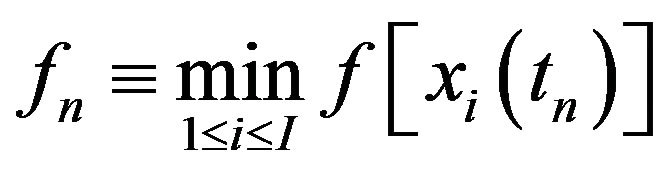 and memorize its value together with the point
  hitting it, i.e.,
 . Repeating the iteration N-times,
 is an approximation value of (3.1) and
 ![]()
such that  is an approximation solution of our scheme.
As ![]() is one of members of swarm
is one of members of swarm  having interactions one and another, the approximate solution
 ![]() may not satisfy the condition
may not satisfy the condition . This means that there is a point
  in a neighborhood of
 ![]() which hits a local minimum of
which hits a local minimum of , i.e.,
 . In this case,
  which can easily be obtained by classical methods (e.g., the steepest descent method) gives a better approximate solution of (3.1) than
![]() .
.
4. Numerical Experiments
We show some numerical experiments to expose the particle’s behavior of our scheme. It is expected that the particles crowd around a point ![]() giving the global minimum of
giving the global minimum of  or are dispersed into a number of neighborhoods of points giving local minimums. The behavior may change heavily depending on the choice of parameters
  and
and![]() .
.
We here use three well known benchmark problems, namely, Problem (3.1) with Sphere function, Rastrigin function and Rosenbrock function. Problem (3.1) with the Sphere function
 (4.1)
(4.1)
is the simplest problem. The optimal point is obviously given by . The following function
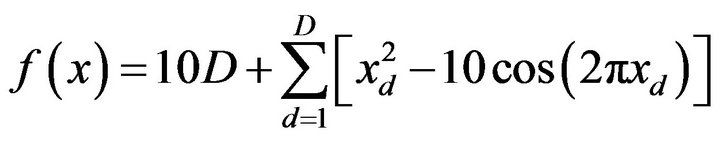 (4.2)
(4.2)
is called the Rastrigin function. Its optimal point is also given by  with the global minimum
 . It is easily seen that this function possesses many local minimums; indeed, at every lattice point,
  has a local minimum. Therefore, Problem (3.1) with function (4.2) is very difficult to treat especially in a high dimension
 . Finally, the Rosenbrock function is formulated by
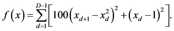 (4.3)
(4.3)
This function takes its global minimum 0 at the lattice point 
As shown below, behavior of the particles depends on the model parameters. We set 
 and
and
 . The step size is fixed by
 and the total step number is
 . As for D, we consider 2-dimensional and 12-dimensional problems.
When , the initial position
  is taken in,
  , where no optional point exists in
 , moreover,
  is far away from the optimal point. In addition, for 2-dimensional Rosenbrock problem, we will take
 , too, because the Rosenbrock function defined by (4.3) is not symmetric with respect to the transformation
 .
.
When , the initial position
  is taken randomly in
 , but it is very difficult to find the optimal point in a higher dimensional search space.
4.1. Sphere Function
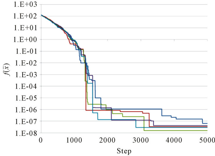
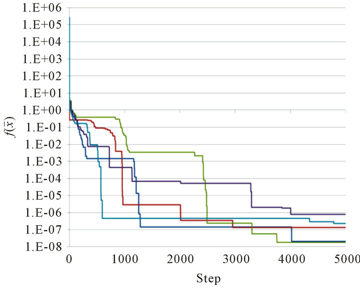
Figure 1 shows the numerical results for Sphere function. The parameters are set as ,
, ;
; ;
; , and
, and . For
. For , the computed result is given by Figure 1(a); similarly for
 , by Figure 1(b).
In the first stage ,
,  decreases rapidly, which means that all the particles strike out for the optimal point 0 in group influenced form the force due to the gradient of
 . In the second stage, since the interaction among particles becomes dominant rather than the potential force, decreasing of the value
  becomes slow. This means that the particles make local searches in a neighborhood of the global optimum. But, the interaction may prevent the optimal particle from attaining exactly the global minimum. So, our method makes it possible to search both wide range and small range by using the same scheme. On the other hand, it is an important problem to find a better combination of parameters in order to have a suitable balance between the global search and the local search.
4.2. Rastrigin Function
Figure 2 shows the numerical results for the Rastrigin
 (a)
(a)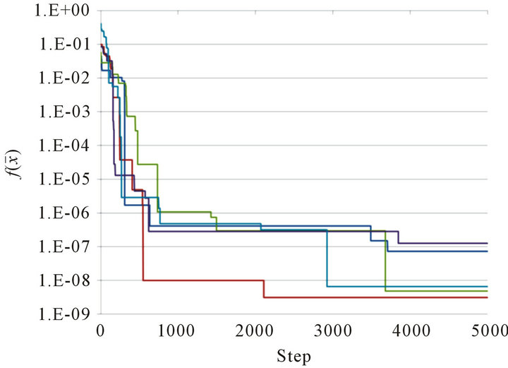 (b)
(b)
Figure 1. Graph of  at Steps 0 ≤ n ≤ 5000 for 5 trials. (a) Sphere function for D = 2; (b) Sphere function for D = 12.
 (a)
(a)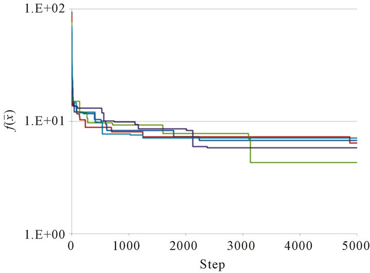 (b)
(b)
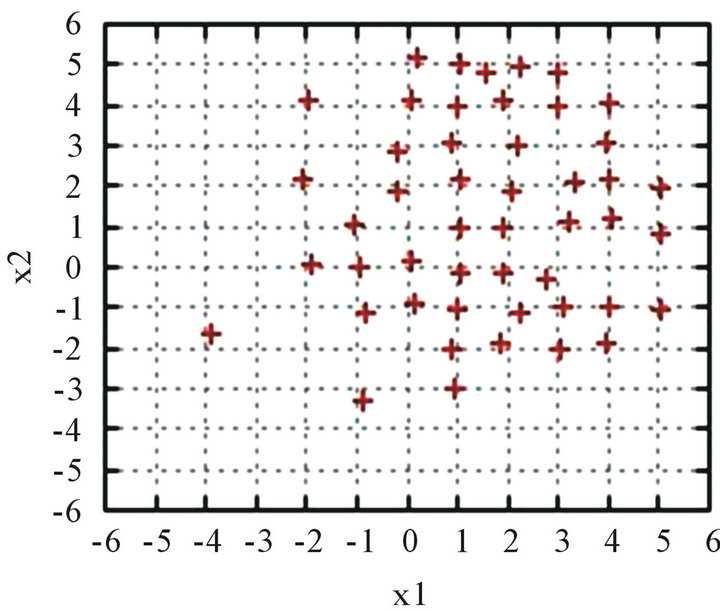
Figure 2. Graph of  at Steps 0 ≤ n ≤ 5000 for 5 trials. (a) Rastrigin function for D = 2; (b) Rastrigin function for D = 12.
function. For D = 2, we set I = 49, ;
; ;
; , and
, and . For
. For  and
and  are replaced by
  and
and , respectively, and the rests are the same as for D = 2. Such a combination yielded the best result in our numerical simulations.
Figures 2(a) and (b) illustrate the graphs of  for 5 trials in the cases D = 2 and D = 12, respectively. Figure 3 then shows the positions of particles at Step
 . (When D = 12, only the first two coordinates are illustrated.) In the 2-dimensional case, many particles reach a neighborhood of the optimal point
  without being trapped by lattice points giving local minima. In the 12-dimensional case, however, no particles can exactly get to the optimal point. But, we see that, for the optimal point
 ![]() of the scheme, most of its coordinates coincide optimally with 0.
of the scheme, most of its coordinates coincide optimally with 0.
In order to measure the total optimality of swarm, we want to consider the total energy defined by
 (a)
(a)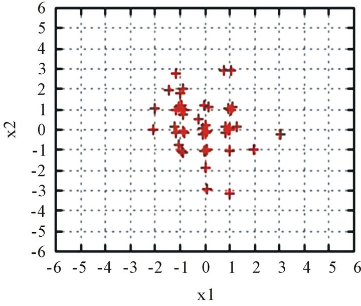 (b)
(b)
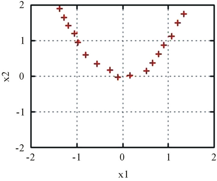
Figure 3. Positions of particles at Step N = 5000. (a) Rastrigin function for D = 2; (b) Rastrigin function for D = 12.
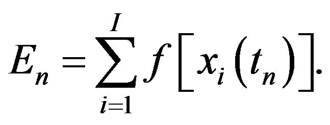
We can say that, if  is small, then most of swarm particles stay in rather better positions and the swarm is in a steady state. To the contrary, if
  is large, then many swarm particles move actively from local minima to others to reach a steady state. Table 1 shows some summation results of
 . As seen by this table, if
 ![]() is too small, namely, the noise is too small, then the swarm is trapped in a steady state of high total energy. To the contrary, if
is too small, namely, the noise is too small, then the swarm is trapped in a steady state of high total energy. To the contrary, if ![]() is sufficiently large, then particles can escape from the trap of local minima and the swarm moves into a state of lower total energy. But if
is sufficiently large, then particles can escape from the trap of local minima and the swarm moves into a state of lower total energy. But if ![]() is too large, then the noise effect disperses swarm particles in every direction to disconnect the interaction among swarm mates. In this simulation, the value
is too large, then the noise effect disperses swarm particles in every direction to disconnect the interaction among swarm mates. In this simulation, the value  is the best one.
4.3. Rosenbrock Function
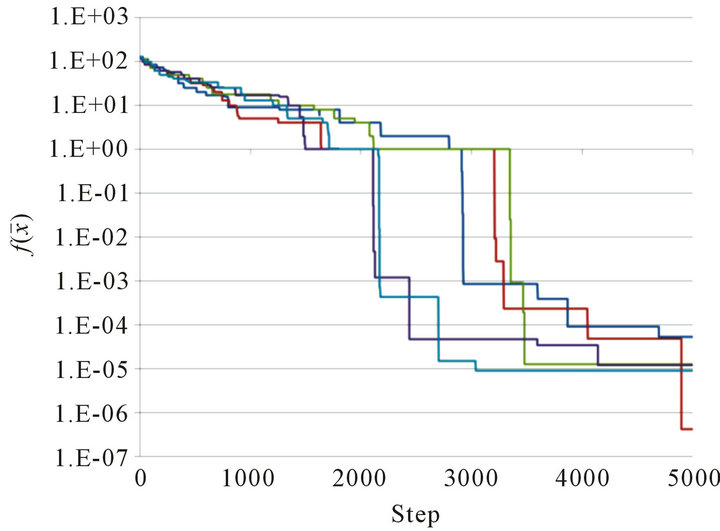
Figure 4 shows the numerical results for the Rosenbrock function. For D = 2, we set ,
,  ,
,  ,
,  , and
, and . The initial positions are set in either
 . For
. For ,
,
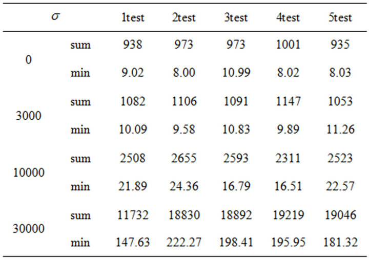
Table 1. Total energy of particles at Step N = 5000.
we set I = 49, w = 0.9,  ,
,  , and
, and 
 . Such a combination provided the best result in our numerical simulations.
Figures 4(a) and (b) illustrate the graphs of  for the 2-dimensional problems with initial positions
 , respectively. Figure 4(c) illustrates the same for the 12-dimensional problem. Figure 5 then shows the positions of particles at Step
 . (When
 , only the first two coordinates are illustrated.) We observe that particles line along a curve drawn on
  by the local minima of
  defined by (4.3).
5. Conclusions
After reviewing the stochastic differential equation model for animal swarming, we have introduced our optimization algorithm directly based on animal swarming behavior, centering, collision avoidance and imperfectness of information-gathering and acting. The optimization function was treated as a potential function and each particle has tendency to move into the most descending direction of the values of the potential function. By these, on one hand, the particles keep on swarming; on the other hand, they search the optimal point globally and locally without being trapped by points giving local minima.
Numerical experiments were performed in order to clarify particle’s behavior of the proposed scheme. We used Sphere function, Rastrigin function and Rosenbrock function. For getting good performance, the parameters of algorithm must be suitably chosen.
Especially,  controls an effective range of how far the interaction among particles is attainable. Meanwhile, r decides the standard distance of any two particles; that is, if the distance of two particles is more than r, then they are attractive each other, on the contrary, if less than r, then they are repulsive. The parameter
 ![]() controls vitality of the swarm. If
controls vitality of the swarm. If ![]() is too small, then the
is too small, then the
 (a)
(a)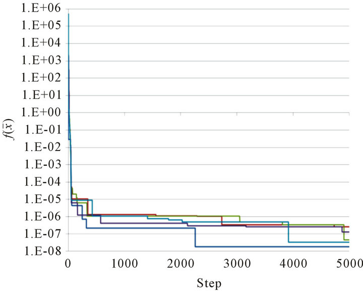 (b)
(b)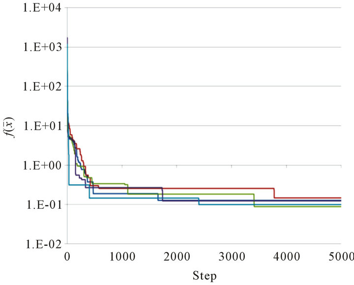 (c)
(c)
Figure 4. Graph of  at Steps 0 ≤ n ≤ 5000 for 5 trials. (a) Rosenbrock function for D = 2 with x0 = K+; (b) Rosenbrock function for D = 2 with x0 = K−; (c)Rosenbrock function for D = 12.
 (a)
(a)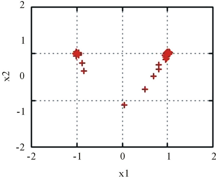 (b)
(b)
Figure 5. Positions of particles at Step N = 5000. (a) Rosenbrock function for D = 2; (b) Rosenbrock function for D = 12.
swarm is easily trapped in a neighborhood of points giving local minima; on the contrary, if too large, then they cannot keep on swarming and they result in searching the optimal point individually. If ![]() is suitably chosen, then the swarm strikes out toward the optimal point making global searching without being trapped by local minima. As shown by numerical examples in 12-dimensional space, such machinery is available even for higher dimensional problems.
is suitably chosen, then the swarm strikes out toward the optimal point making global searching without being trapped by local minima. As shown by numerical examples in 12-dimensional space, such machinery is available even for higher dimensional problems.
Our optimization method devised on the basis of animal swarming may be applicable to various optimization problems presented from the real world. In those problems, it may be unknown whether the optimization function is of class  or not, or even if so, its gradient may not be easily computed. For further such applications, we have therefore to combine our method with some methods of numerical differentiations or those of differentiating non smoothing functions numerically using functional values alone.
REFERENCES
- Kennedy and R. Eberhart, “Particle Swarm Optimization,” Proceedings of IEEE International Conference Neural Networks, Perth, 27 November-1 December 1995, 1942-1948.
- D. Bratton and J. Kennedy, “Defining a Standard for Particle Swarm Optimization,” IEEE Swarm Intelligence Symposium, Honolulu, 1-5 April 2007, pp. 120-127.
- H. Liu, A. Abraham and W. Zhang, “A Fuzzy Adaptive Turbulent Particle Swarm Optimization,” International Journal of Computer Applications, Vol. 1, No. 1, 2007, pp. 39-47. doi:10.1504/IJICA.2007.013400
- S. He, Q. Wu, J. Wen, J. Sanuders and R. Paton, “A Particle Swarm Optimizer with Passive Congregation,” Biosystems, Vol. 78, 2004, pp. 135-147. doi:10.1016/j.biosystems.2004.08.003
- M. Eslami, H. Shareef, M. Khajehzadeh and A. Mohamed, “A Survey of the State of the Art in Particle Swarm Optimization,” Research Journal of Applied Science, Engineering and Technology, Vol. 4, 2012, pp. 1181-1197.
- J. S. Camazine, J. L. Deneubourg, N. R. Franks, J. Sneyd, G. Theraulaz and E. Bonabeau, “Self-Organization in Biological Systems,” Princeton University Press, Princeton, 2001.
- C. W. Reynolds, “Flocks, Herds, and Schools: A Distributed Behavioral Model,” Computer Graphics, Vol. 21, No. 4, 1987, pp. 25-34. doi:10.1145/37402.37406
- T. Uchitane, T. V. Ton and A. Yagi, “An Ordinary Differential Equation Model for Fish Schooling,” Scientiae Mathematicae Japonicae, Vol. 75, 2012, pp. 339-350.
- B. Øksendal, “Stochastic Differential Equations,” Springer, Berlin, 2007.