Advances in Remote Sensing
Vol.06 No.01(2017), Article ID:73549,17 pages
10.4236/ars.2017.61002
Comparative Study among Different Semi-Empirical Models for Soil Salinity Prediction in an Arid Environment Using OLI Landsat-8 Data
A. El-Battay1, A. Bannari1, N. A. Hameid1, A. A. Abahussain2
1Department of Geoinformatics, College of Graduate Studies, Arabian Gulf University, Manama, Kingdom of Bahrain
2Natural Resources and Environment Department, College of Graduate Studies, Arabian Gulf University, Manama, Kingdom of Bahrain

Copyright © 2017 by authors and Scientific Research Publishing Inc.
This work is licensed under the Creative Commons Attribution International License (CC BY 4.0).
http://creativecommons.org/licenses/by/4.0/


Received: November 28, 2016; Accepted: January 15, 2017; Published: January 18, 2017
ABSTRACT
Salt-affected soils, caused by natural or human activities, are a common environmental hazard in semi-arid and arid landscapes. Excess salts in soils affect plant growth and production, soil and water quality and, therefore, increase soil erosion and land degradation. This research investigates the performance of five different semi-empirical predictive models for soil salinity spatial distribution mapping in arid environment using OLI sensor image data. This is the first attempt to test remote sensing based semi-empirical salinity predictive models in this area: the Kingdom of Bahrain. To achieve our objectives, OLI data were standardized from the atmosphere interferences, the sensor radiometric drift, and the topographic and geometric distortions. Then, the five semi-empirical predictive models based on the Normalized Difference Salinity Index (NDSI), the Salinity Index-ASTER (SI-ASTER), the Salinity Index-1 (SI-1), the Soil Salinity and Sodicity Index-1 and Index-2 (SSSI-1 and SSSI-2), developed for slight and moderate salinity in agricultural land, were implemented and applied to OLI image data. For validation purposes, a fieldwork was organized and different important spots-locations representing different salinity levels were visited, photographed, and localized using an accurate GPS (σ ≤ ±30 cm). Based on this a priori knowledge of the soil salinity, six validation sites were selected to reflect non-saline, low, moderate, high and extreme salinity classes, descriptive statistics extracted from polygons and/or transects over these sites were used. The obtained results showed that the models based on NDSI, SI-1 and SI-ASTER all failed to detect salinity bounds for both extreme salinity (Sabkhah) and non-saline conditions. In Fact, NDSI and SI- ASTER gave respectively only 35% dS/m and 25% dS/m in extreme salinity validation site, while SI-1 and SI-ASTER indicated 38% dS/m and 39% dS/m in non-saline validation site. Therefore, these three models were deemed inadequate for the study site. However, both SSSI-1 and SSSI-2 allowed a detection of the previous salinity bounds and furthermore described similarly and correctly the urban-vegetation areas and the open-land areas. Their predicted EC is around 10% dS/m for non-saline urban soil, about 25% dS/m for low salinity urban-vegetation soil, approximately 30% to 75% dS/m, respectively, for moderate to high salinity soils. SSSI-2 based semi-empirical salinity models was able to differentiate the high salinity versus extreme salinity in areas where both exist and was very accurate to highlight the pure salt where SSSI-1 has reach saturation for both salinity classes. In conclusion, reliable salinity map was produced using the model based on SSSI-2 and OLI sensor data that allows a better characterization of the soil salinity problem in an Arid Environment.
Keywords:
Soil Salinity, Spectral Indices, Semi-Empirical Models, Arid Land, Landsat-OLI

1. Introduction
Soil salinity is a major and serious problem especially in arid and semi-arid environment. Excess of salt concentration in soils affects significantly plant growth, crop and palms trees production, soil and water quality, and consequently soil erosion and land degradation [1] [2] [3] . Its impacts affect not only the environment, but also the economic aspects [4] . The spatial and temporal variability of soil salinity over the landscape is controlled by different factors [5] . These included soil variables (soil composition, structure and texture, permeability, organic matter, geological formation, water table depth, ground and irrigation water quality, and the salt content), topographical variables (elevations, slopes and orientations), climatic variables under climate change pressure (precipitations, temperature, and evapotranspiration), and fields management practices (irrigation and drainage) [6] . Therefore, it is important to monitor and map salinity at an early stage to prevent future increase in soil. Definitely, accurate information about the extent, magnitude, and spatial distribution of salinity will help to create sustainable development of natural resources [7] . Ground-based electrical conductivity (EC) measurements of soil are generally the most effective methods for quantification of soil salinity. Unfortunately, these methods are expensive, time consuming, and need considerable human resources for field sampling and laboratory analysis. Remote sensing and GIS offer advantages to the ground- based methods because they make it possible to map accurately vast areas subject to soil salinity hazard in space and time [8] .
Soil salinity is highly dynamic, varies considerably in time and in space, and modify temporarily or permanently the state of the surface and of the soils below [9] . The adoption of suitable management methods in areas vulnerable to salinity can slow the salinization processes and even to reverse them completely. Without adequate information, mitigation measures and actions cannot be applied to the affected soils and damage becomes irreversible if left unattended for long time. Therefore, in order to properly manage the situation; salinity information must be not only accurate and reliable, but also up-to-date [10] . In affected areas, farmers, soil managers, scientists and agricultural engineers need accurate and reliable information on the nature, scope or extent, severity and spatial distribution of the salinity against which they could take appropriate measures [11] [12] . Remedial actions require reliable information to help set priorities and to choose the type of action that is most appropriate in each situation [11] . Consequently, it is important to monitor and map soil salinity at an early stage to prevent future increase of salinity in soil. Definitely, accurate information about the extent, magnitude, and spatial distribution of salinity will help create sustainable development of natural resources [7] . Knowing when, where and how salinity may occur is very important to the sustainable development of any irrigated production system especially in arid and semi-arid environment.
Different spectral salinity indices have been proposed in the literature for the detection and identification of probable saline soils. Khan et al. [13] proposed three spectral indices for the identification of salinity in Pakistan using predominantly bands 3 and 4 of the LISS-II sensor of the IRS-1B platform: Brightness Index (BI), Normalized Difference Salinity Index (NDSI) and Salinity Index (SI). Among these three indices, the authors found that the NDSI showed the most promises in the extraction of different salinity classes in a semi-arid environment using satellite data and ground truth data. Using ground based spectral data; Al-Khaier (2003) developed the Salinity Index using bands 4 and 5 of ASTER sensor (SIASTER). It was reported that this index detect accurately the soil salinity phenomenon in semi-arid irrigated agricultural regions of Syria. A cooperative project between India and the Netherland [14] proposed a methodology for the cartography of soil salinity and waterlogging in irrigated cropped land in a semi-arid region of India. After analyzing different remote sensing techniques, this project recommended three different Salinity Indices using Landsat-TM Bands (4, 5 and 7): SI-1, SI-2 and SI-3. These three indices were developed using surface radiative properties data, biomass depression and moisture indicators. Exploiting field soil sampling, laboratory analysis (EC), and ground spectroradiometric data to simulate the EO-1 ALI sensor data, [15] demonstrated that the short waves infrared (SWIR) are more sensitive than other bandwidths to different degrees of salinity and sodicity, especially for slight and moderate levels. They proposed two indices: Soils Salinity and Sodicity Indices 1 and 2 (SSSI-1 and SSSI-2). These indices are particularly well suited to the identification of low and medium levels of salinity and sodicity over irrigated agricultural land in semi-arid environment. Furthermore, considering different soil sample with diverse salinity content, all these spectral salinity indices were derived from the spectroradiometric measurements. Then, they were correlated to EC extracted from a saturated soil paste using a second order regression analysis to establish semi-empirical models for soil salinity prediction. Among the considered nine derived predictive semi-empirical models, in this research we consider only five models that show significant correlation coefficient (R2 ≥ 0.70) according to the data simulation, laboratory analysis and statistical investigation. Detailed description of the steps leading this development can be found in [7] [15] .
This research investigate the performance of five different semi-empirical predictive models for soil salinity spatial distribution mapping in the arid environment of Kingdom of Bahrain using OLI Landsat-8 image data. This is the first attempt to test remote sensing based semi-empirical salinity predictive models in this area; the Kingdom of Bahrain. Hence, in this study salinity spectral indices originally well suited to the identification of low and medium levels of salinity and sodicity over irrigated agricultural land in semi-arid environment will be used in arid environment where salinity may reach extreme levels (Sabkhah). In the total absence for the study area of any remote sensing based salinity mapping technique, this study aims to test, retain and propose some remote sensing based salinity semi-empirical predictive models suitable for it.
2. Material and Methods
2.1. Study Site
The Kingdom of Bahrain is a group of islands located in the Arabian Gulf, east of Saudi Arabia and west of Qatar (26˚00'N, 50˚33'E), Figure 1. The archipelago comprises 33 islands, with a total land area of about 765.30 km2 [16] . According to the aridity criteria and consequently to great variations in climatic conditions, Bahrain has an arid to extremely arid environment [17] . The Island is characterized by high summer temperatures around 45˚C (June-September) and an average of 17˚C approximately in winter (December-March). The rainy season runs from November to April, with an annual average of 72 mm, sufficient only to support the most drought resistant desert vegetation. Mean annual relative humidity is over 70% due to the surrounding Arabian Gulf waters, and the annual average potential evapotranspiration rate is 2099 mm [18] . Geologically, Bahrain is characterized by Eocene and Neocene rocks, which are partly covered by Quaternary sediments and a complex of Pleistocene deposits. The dominant rocks are limestone and dolomitic-limestone with subsidiary marls and shales. The leading structure is the north-south axis of the main dome, with minor cross folds predominantly tilting from northeast to southwest. The beds are gently inclined towards the coast from the center of the main island. The fringes of Bahrain are covered by more recent marine and Aeolian sand dunes, which were derived from the Arabian land connection across the present Arabian Gulf [19] .
2.2. Methodology Flowchart and Salinity Models
This research investigate the performance of five different semi-empirical pre-

Figure 1. Study site, Kingdom of Bahrain.
dictive models for soil salinity spatial distribution mapping in an arid environment using OLI Landsat-8 image data. To achieve our objectives, these data were atmospherically corrected, sensor radiometric drift calibrated, and distortions of topography and geometry corrected using a digital elevation model (DEM). Then, five predictive semi-empirical models based on the Normalized Difference Salinity Index (NDSI) [13] , the Salinity Index-ASTER (SI-ASTER) [12] , the Salinity Index-1 (SI-1) [14] , the Soil Salinity and Sodicity Index-1 and Index-2 (SSSI-1 and SSSI-2) [15] were implemented and applied to OLI image data. Finally, for validation purposes, a fieldwork was organized and different important spots-lo- cations representing different salinity levels were visited, photographed, and localized using an accurate GPS (σ ≤ ±30 cm). Based on a priori knowledge of the soil salinity class’s characteristics, descriptive statistics extracted from polygons and/or transects over the selected validation sites were used. Figure 2 summarized the used methodology that will be discussed in details in the subsequent section.
2.3. OLI Landsat-8 Data and Processing
Since 1972, the Landsat scientific collaboration program between the USGS and NASA constitute the continuous record of the Earth’s surface reflectivity from space [20] . Indeed, the Landsat satellites series (from MSS to OLI) support more
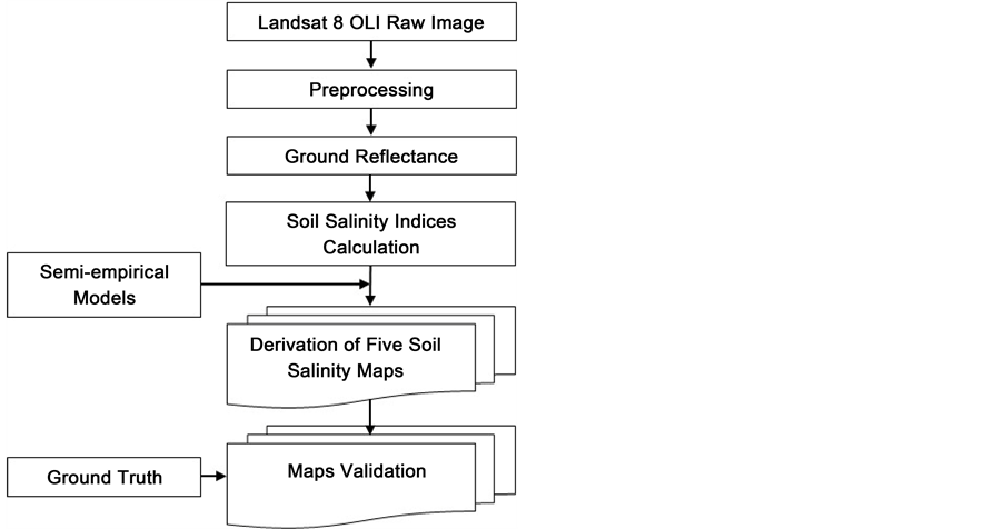
Figure 2. Methodology flowchart.
than four decades a global moderate resolution data collection, distribution and archive of the Earth’s continental surfaces [21] to support research, applications, andclimate change impact analysis at the global, the regional and the local scales. The OLI sensor on board of the Landsat-8, collects land-surface reflectivity in the visible, near infrared, and shortwave infrared wavelength regions as well as a panchromatic band, similarly to ETM+ sensor. However, the passes-bands and relative responsivity are narrower than that of the ETM+ in order to minimize atmospheric absorption features [22] . Two new spectral bands have been added: a deep blue visible shorter wavelength (band 1: 0.433 - 0.453 μm) designed specifically for water resources and coastal zone investigation, and a new infrared channel (band 9: 1.360 - 1.390 μm) for the detection of cirrus clouds in the atmosphere. The OLI images have 15 meter in panchromatic and 30 meter in multi-spectral spatial resolutions covering approximately 185 by 185 km. The entire Earth is imaged each every 16 days due to Landsat-8 near-polar circular orbit at 705 km [23] . For this research, the OLI image was acquired on 5th April 2014 over the Kingdom of Bahrain.
According to the OLI image preprocessing steps, we consider sensor radiometric drift, atmospheric corrections, and geometric and topographic rectification. Drift of the sensor radiometric calibration is a necessary step, which consists of correcting artifacts affecting the sensor in order to extract precise and reliable information from an image [24] . Relative calibration is a normalization and harmonization of the data received from the different detectors of OLI sensor. Absolute calibration allows the transformation of the digital number, which is measured at the top of the atmosphere into apparent reflectance. Then, for the atmospheric correction (absorption by gases and scattering by aerosols and molecules), the ATCOR model implemented in PCI-Geomatica [25] was used. The input parameters for this radiative transfer code considering the image are

Table 1. Input parameters for ATCOR radiative transfer code.
Note: ASL, above sea level; GMT: Greenwich Mean Time; ppm, parts per million.
summarized in Table 1. In order to preserve the radiometric integrity of the image, drift of the sensor radiometric calibration and atmospheric effects were combined and corrected in one-step to transform the digital number to the ground reflectance [26] .
For geometric and topographic distortions rectification, second-degree polynomial transformation cannot eliminate the distortions caused by the relief and the shadow impact, because the intersection of the field of view with the ground produces pixels with variable size following the slope and aspect [27] . Indeed, it is necessary to have an altitude value for any point on the image, namely DEM, in order to ortho-rectify rigorously the images [28] . According to Burrough and McDonnell [29] , the DEM must be in the size range of the image or higher spatial resolution to provide an ortho-image with good precision. In this research, we conducted an ortho-rectification using Advanced Space-borne Thermal Emis- sion and Reflection Radiometer (ASTER) DEM with 30-m pixel size and the “Rational-Function” model implemented in Ortho-Engine module of PCI-Geo- matica. This step enables corrections of the parallax effect at the spatial arrange- ment of pixels along the line of the sweeping and disruptive effects caused by shadow and by topographic variability. To preserve the images radiometric integrity, geometric corrections have been combined into a single step with the correction of topographic effects [30] .
Once the preprocessing is done and DN are converted into ground reflectance values, soil salinity indices and therefore the five predictive semi-empirical models considered in this study were computed according to Equations ((1) to (5)). In fact, the established mathematical equations for these models that are considered in this research are the following [7] [15] :
(1)
(2)
(3)
(4)
(5)
where:
ρRED: ground reflectance in the red band of OLI sensor,
ρNIR: ground reflectance in the near-infrared band of OLI sensor,
ρSWIR-1: ground reflectance in the shortwave infrared band of OLI sensor covering (band 6), and
ρSWIR-2: ground reflectance in the shortwave infrared band of OLI sensor (band 7).
2.4. Validation Process
For validation purposes, six hot-spot locations over Bahrain territory were selected based on their degrees of salinity, i.e. ability to be easily used as a reference to assess the performance of the used models. Figure 3 depicts the location of each validation site that are labeled A, B, C, D, E and F. Site A is located in northwest of the study area that is the most important agricultural fields in Bahrain with low to moderate salinity (Figure 4(a) and Figure 4(b)) classes. The

Figure 3. Location of validation sites in Landsat OLI Image of 5 April 2014 (RGB: 5, 4, 3) over Bahrain (left) and extent of validations sites (Right).

Figure 4. Agricultural farms with low to moderate salinity ((a) and (b)), urban without salinity ((c) and (d)), open land-bare soil with moderate to high salinity ((e) and (f)), and Sabkhah with extreme salinity ((g) and (h)).
low salinity area is predominantly a mixture of silts, sandy loam and loamy sand, and categorized as good land for agriculture, while the moderate salinity zone is composed totally from sand with low potential for agriculture. Site B consisting of soil without salinity (non-saline), located in dense urban environment and transportation network in Manama city (manmade infrastructure), and with very limited vegetation cover and open areas covering a total surface of 4.2 km2 (Figure 4(c) and Figure 4(d)). In Figure 3, the used false color composite allows to discriminate clearly vegetation land cover in red color and urban areas in dark grey. This site is used as a reference for non-saline soil class, and therefore any model indicating a significant salinity in this area is discarded. Site C highlighted the contrast between urban and agricultural-farms (non-saline and low-moderate salinity classes), located in the central Bahrain towards the west. It is situated between urban area and the elongated palm-agricultural farms besides it. In this area (C), transect of 2.5 km was selected as shown in Figure 3 and the models must stressed the contrast between the urban areas (non-saline class) and the low-moderate salinity in the palm trees farms.
Site D is characterized with moderate to high salinity class highlighting the contrast between urban and open-land (Figure 4(e) and Figure 4(f)). The soils of this area are calcareous to highly calcareous whit high gypsum and calcium carbonate content, poor in organic matter (˂1%), deficient in micronutrient, and low fertility potential. Additionally, the preponderance in carbonate and the presence of bicarbonate are responsible on the sodic aspect in the soils [19] . In this area (D), transect of 4.8 km was used to test the models discrimination capability between these salinity classes. Finally, sites E and F covering each one approximately 3 km2 and representing, respectively, the extremely (Figure 4(g) and Figure 4(h)) and very high salinity classes. Site E is located in Sabkhah with extreme salinity caused by seawater intrusion, while the high salinity of the site F is caused by the geological nature of rocks. Figure 4(g) and Figure 4(h) shown clearly that in some limited areas of the Sabkhah pure salt crystals are accumulated in the surface with a thickness of up to 15 cm, while salt crust is observed in other parts. The soil in this site is composed of carbonate-rich-silts with gypsiferous sands. These two sites are crucial to determine the capacity of the each model to discriminate between these classes. Models that fail to detect the extreme and high salinity in these sites (E and F) will be dimmed directly as underperforming. Not only these two sites played a crucial role into discriminating between the five salinity models in term of detecting extreme salinity, they also allow in the affirmative if the model reach saturation or not.
To summarize the validation process for the performance of the five salinity models retained in this study, sites B (non-saline), E and F (very high and extreme salinity) will be used as a first prescreening where any model failing to discriminate any of the non-saline and extreme saline sites is discarded immediately. Models passing that first criterion, if any, are then analyzed further using sites C and D to test their ability to highlight the contrast of salinity between urban/vegetation and urban/open areas land covers.
3. Results and Discussion
Figure 5 and Figure 6 present the salinity maps derived from the five used semi- empirical predictive models. Note that all the derived maps were produced using the same pseudo-color ramp scale. Based on Taylor [31] soil salinity classification scale among non-saline to extreme salinity classes, we adopted a normalized scale for the predictive models EC values between 0% and 100% dS/m, respec-
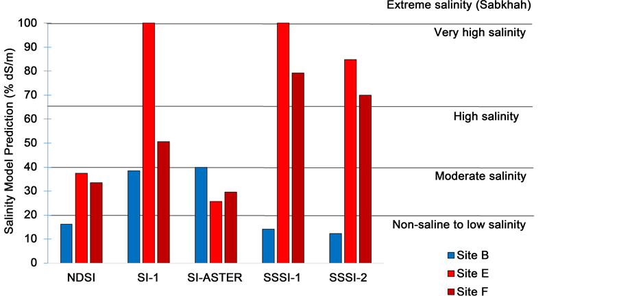
Figure 5. Results of all five models over validation sites B, E and F.
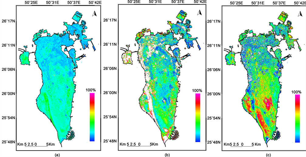
Figure 6. Derived salinity maps using semi-empirical models based on NDSI (a), SI-1 (b) and SI-ASTER (c).
tively, for non-saline and extreme salinity (Sabkhah). Hence, in the maps, blue color means non-saline to low salinity areas with very low EC values (EC ≤ 20%). Green and yellow represent progressively increasing levels of salinity from moderate (20% ˂ EC ≤ 40%) to high (40% ˂ EC ≤ 65%) classes. Whereas, the purple and red colors represent very high level of salinity (EC > 65% ds/m), while white color means signal saturation (EC ≥ 100%) areas with extreme salinity conditions (Sabkhah).
Based on the validation criteria stated above, Table 2 and Figure 5 represent the main results produced using the histogram statistics analysis over the sites B (non-saline), and E and F (Sabkhah). It shows the estimated EC mean and standard deviation values predicted for each site using the five considered models. Figure 6(a) and Table 2 values show that the model based on NDSI has failed to detect the extreme and very high salinity classes in both sites E and F, while it did detect the low salinity in site B. The model based on SI-1 (Figure 6(b)) detected only the high salinity in site E (Sabkhah) but, unfortunately, it failed to characterize high salinity of the site F (caused by the geological nature of rocks). Moreover, it represent the agricultural fields (site B) inappropriately as a Sabkhah with saturated signal (EC > 100%). Furthermore, the model based on SI-ASTER (Figure 6(c)) expressed the worst results, it failed to perform in all three validation sites. Indeed, the Sabkhah and high salinity were mapped as a non-saline soil, while a portion of the moderate salinity class has been misrepresented as an extreme salinity class (Sabkhah). On the other hand, both models based on SSSI-1 and SSSI-2 were able to detect the low salinity class in site B (urban area, EC ˂ 20%), and the extreme and very high salinity classes (EC > 100%) in both sites E and F (Figure 7 and Table 2). However, Figure 7(a) shows
Table 2. Results of the first criterion of validation.
 (a) (b)
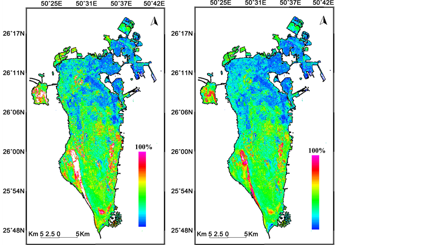
Figure 7. Derived salinity maps using semi-empirical models based on SSSI-1 (a) and SSSI-2 (b).
that the model based on SSSI-1 has oversaturated above the site E (EC ≈ 145.24%), while SSSI-2 was able to highlight smoothly the very high salinity in site E before reaching saturation in spots of pure salt (Sabkhah). In addition, the model built on SSSI-1 overclassified all agricultural fields as a moderate saline soil class with- out sensitivity to low salinity farms. Whereas, the model based on SSSI-2 index discriminated significantly between low and moderate saline farms. Consequent- ly, models based on NDSI, SI-1, SI-ASTER were discarded for further analysis, and only ones based on SSSI-1 and SSSI-2 were retained.
Figure 8 shows the transect profiles of salinity values obtained by the two models based on SSSI-1 and SSSI-2 over the sites C and D. Considering site C, transect highlighted the contrast between urban area and agricultural-farms that are non-saline and low-moderate salinity classes. Figure 8(a) shows that the both model characterize similarly the dense urban area (non-saline class), the EC values remain under 20% dS/m. However, the low and moderate salinity classes

Figure 8. Salinity profiles over site C ((a) up) and site D ((b) down) using semi-empirical models based on SSSI-1 and SSSI-2.
in agricultural area are significantly overestimated with SSSI-1 model, EC between 30% and 60% dS/m. This confirms the tendency of SSSI-1 model to exaggerate the salinity prediction, and that is why it reaches saturation more often compared to SSSI-2 model. This describe appropriately these two classes, always the EC values remain between 20% and 40% dS/m. Otherwise, the transect over the site D highlighted the contrast between urban-vegetation areas with non-sa- line to moderate salinity classes and open-land with moderate to high salinity classes (Figure 8(b)). The two models transect-profiles described similarly and correctly the urban-vegetation areas and the open-land areas. The predicted EC is around 10% dS/m for non-saline urban soil, about 25% dS/m for low salinity urban-vegetation soil, approximately 30% to 75% dS/m for moderate to high salinity soils, respectively.
Generally, both models performed well to detect the very high salinity class and non-saline soil with a tendency of the SSSI-1 to amplify salinity response and hence reach saturation quickly compared to SSSI-2. This was further confirmed in the agricultural field for moderate salinity where SSSI-2 model remained consistent, while SSSI-1 based model classified it as high salinity area. Furthermore, SSSI-2 based model was able to differentiate the high salinity versus extreme salinity in areas where both exist and was very accurate to highlight the pure salt where it has reach saturation.
Therefore, the model based on SSS-2 performed well and passed all the validation tests and is recommended to be used for the study area. In fact, if to be used in open areas where very high or even extreme levels of salinity are observed such as in Sabkhah areas, SSSI-1 has reached saturation very quickly, especially when tested in site E for which a very good field expertise exist. At the opposite, SSSI-2 based model was able to differentiate in the same area two classes of salinity and was very accurate to highlight the pure salt where it has reach saturation. In conclusion, reliable salinity map was produced using the model based on SSSI-2 and OLI sensor data that allows a better characterization of the soil salinity problem in an Arid Environment.
4. Conclusion
The main aim of this research was to assess the potential of OLI sensor on board the Landsat-8 satellite for the potential discrimination and mapping of salt-af- fected soils in an arid land. Non-saline soil, low, moderate, high, very high and extreme salinity (Sabkhah) classes were considered. Moreover, the potentials and limits of five semi-empirical predictive models developed previously for soil salinity detection and mapping were compared using six selected validation sites. Obtained results showed that the models based on NDSI, SI-1 and SI-ASTER all failed to detect salinity bounds for very high and extreme (Sabkhah) salinity, and non-saline classes. The SSSI-1 based model has a tendency to overestimate strongly the salinity response and reaches saturation quickly (EC ≈ 145.24%) causing confusion among high, very high and extreme salinity classes. In addition, it overclassified all agricultural fields as a moderate saline soil class without sensitivity to low salinity farms. On the other hand, the model based on SSSI-2 was able to highlight gradually all the salinity classes with a very good conformity with the ground truth, highlighting all the six major salinity classes. Therefore, salinity semi-empirical predictive models based on SSSI-2 salinity indices is very suitable to know where salinity occur and it’s dynamic in space and time in the arid environment of the kingdom of Bahrain. Moreover, short waves infrared (SWIR) salinity indices are more sensitive than other bandwidths to different degrees of salinity and sodicity, for slight and moderate levels [15] but also in this study using these indices with OLI data was effective to detect high, very high and extreme salinity levels. A next step will be to collect field samples and calibrate the SSSI-2 based semi-empirical model to quantitatively predict EC, this information is very important for continuously monitoring salinity changes using OLI Landsat-8 Data over the kingdom of Bahrain.
Acknowledgements
The authors would like to thank the Arabian Gulf University for financial support. They acknowledge the GLOVIS-USGS Gate, NASA, for OLI Landsat-8 data. Finally, we would also like to thank the anonymous reviewers for their constructive rectifications and comments.
Cite this paper
El-Battay, A., Ban- nari, A., Hameid, N.A. and Abahussain, A.A. (2017) Comparative Study among Different Semi-Empirical Models for Soil Salinity Pre- diction in an Arid Environment Using OLI Landsat-8 Data. Advances in Remote Sensing, 6, 23-39. https://doi.org/10.4236/ars.2017.61002
References
- 1. Zinck, J.A. and Metternicht, G. (2009) Soil Salinity and Hazard. In: Metternicht, G. and Zinck, J.A., Eds., Remote Sensing of Soil Salinization: Impact on Land Management, CRC Press Taylor and Francis Group, Boca Raton, 3-20.
- 2. Alhammadi, M.S. and Kurup, S.S. (2012) Impact of Salinity Stress on Date Palm (Phoenix dactylifera L.)—A Review. In: Sharma, P., Ed., Crop Production Technologies, In Tech, 169-178.
- 3. Allbed, A. and Kumar, L. (2013) Soil Salinity Mapping and Monitoring in Arid and Semi-Arid Regions Using Remote Sensing Technology: A Review. Advances in Remote Sensing, 2, 373-385. https://doi.org/10.4236/ars.2013.24040
- 4. Naifer, A., Al-Rawahy, S.A. and Zekri, S. (2011) Economic Impact of Salinity: The Case of Al-Batinah in Oman. International Journal of Agricultural Research, 6, 134-142. https://doi.org/10.3923/ijar.2011.134.142
- 5. Allbed, A., Kumar, L. and Sinha, P. (2014) Mapping and Modeling Spatial Variation in Soil Salinity in the Al Hassa Oasis Based on Remote Sensing Indicators and Regression Techniques. Remote Sensing, 6, 1137-1157. https://doi.org/10.3390/rs6021137
- 6. Douaik, A., Meirvenne, M. and Toth, T. (2008) Stochastic Approaches for Space-Time Modeling and Interpolation of Soil Salinity. In: Metternicht, G. and Zinck, J.A., Eds., Remote Sensing of Soil Salinization: Impact on Land Management, CRC Press Taylor and Francis Group, Boca Raton, 273-289. https://doi.org/10.1201/9781420065039.ch14
- 7. Bannari, A., Guédon, A.M. and El-Ghmari, A. (2016) Mapping Slight and Moderate Saline Soils in Irrigated Agricultural Land Using Advanced Land Imager Sensor (EO-1) Data and Semi-Empirical Models. Communications in Soil Science and Plant Analysis Journal, 47, 1883-1906. https://doi.org/10.1080/00103624.2016.1206919
- 8. Metternicht, G. and Zinck, J.A. (2009) Remote Sensing of Soil Salinization: Impact on Land Management. CRC Press Taylor and Francis Group, Boca Raton, 374.
- 9. Mougenot, B., Pouget, M. and Epema, G. (1993) Remote Sensing of Salt Affected Soils. Remote Sensing Review, 7, 241-259. https://doi.org/10.1080/02757259309532180
- 10. Smedema, L.K. (1995) Salinity Control in Irrigated Land: Use of Remote Sensing techniques in irrigation and Drainage. Proceeding of the Expert Consultation, Session 3-Drainage and Salinity Monitoring and Control. Montpellier, 2-4 November 1993, FAO, 141-150.
- 11. Metternicht, G.I. and Zinck, J.A. (2003) Remote Sensing of Soil Salinity: Potentials and Constraints. Remote Sensing of the Environment, 85, 1-20. https://doi.org/10.1016/S0034-4257(02)00188-8
- 12. Al-Khaier, F. (2003) Soil Salinity Detection Using Satellite Remotes Sensing. Master Thesis, International Institute for Geo-Information Science and Earth Observation, Enscheda, 61 p.
- 13. Khan, N.M., Rastoskuev, V.V., Shalina, E.V. and Sato, Y. (2001) Mapping Salt-Affected Soils Using Remote Sensing Indicators—A Simple Approach with the Use of GIS IDRISI. Proceedings of the 22th Asian Conference on Remote Sensing, Singapore, 5-9 November 2001, 5 p.
- 14. IDNP (2002) Indo-Dutch Network Project: A Methodology for Identification of Water-logging and Soil Salinity Conditions Using Remote Sensing. Central Soil Salinity Research Institute, Karnal, 78 p.
- 15. Bannari, A., Guedon, A.M., El-Harti, A., Cherkaoui, F.Z. and El-Ghmari, A. (2008) Characterization of Slight and Moderate Saline and Sodic Soils in Irrigated Agricultural Land Using Simulated Data of ALI (EO-1) Sensor. Communications in Soil Science and Plant Analysis Journal, 39, 2795-2811. https://doi.org/10.1080/00103620802432717
- 16. CIO (2013) Population, Housing, Buildings, Establishments and Agriculture Census: Census Summary Result 2010. Central Informatics Organization, Isa Town, 21 p.
- 17. Elagib, N.A. and Addin, A.S.A. (1996) Climate Variability and Aridity in Bahrain. Journal of Arid Environments, 36, 405-419. https://doi.org/10.1006/jare.1996.0237
- 18. FAO (2015) Bahrain: Geography, Climate and Population. http://www.fao.org/nr/water/aquastat/countries_regions/bahrain/index.stm
- 19. Doornkamp, J.C., Brunsden, D. and Jones, D.K.C. (1980) Geology, Geomorphology and Pedology of Bahrain. Geo-Abstracts Ltd., University of East Anglia, Norwich, 443 p.
- 20. Bannari, A., Teillet, P.M. and Landry, R. (2004) Comparaison des réflectances des surfaces naturelles dans les bandes spectrales homologues des capteurs TM de Landsat-5 et TME+ de Landsat-7. Revue Télédétection, 4, 263-275.
- 21. NASA (2015) Operational Land Imager (OLI). http://landsat.gsfc.nasa.gov/?p=5447
- 22. Wulder, M.A., White, J.C., Masek, J.G., Dwyer, J. and Roy, D.P. (2012) Continuity of Landsat Observations: Short Term Considerations. Remote Sensing of Environment, 115, 747-751. https://doi.org/10.1016/j.rse.2010.11.002
- 23. NASA (2014) Landsat-8 Instruments. http://www.nasa.gov/mission_pages/landsat/spacecraft/index.html
- 24. Bannari, A., Teillet, P.M. and Richardson, G. (1999) Nécessité de l'étalonnage radiométrique et standardisation des données de télédétection. Journal Canadien de Télédétection, 25, 45-59.
- 25. PCI Geomatics (2014) Using PCI Software. Richmond Hill, 540 p.
- 26. Teillet, P.M. and Santer, R.P. (1991) Terrain Elevation and Sensor Altitude Dependence in Semi-Analytical Atmospheric Code. Canadian Journal of Remote Sensing, 17, 36-44.
- 27. Bannari, A., Morin, D., Bénié, G.B. and Bonn, F. (1995) A Theoretical Review of Different Mathematical Models of Geometric Corrections Applied to Remote Sensing Images. Remote Sensing Reviews, 13, 27-47. https://doi.org/10.1080/02757259509532295
- 28. Caloz, R., Blaser, T.J. and Willemin, G. (1993) Création d’ortho-image à l’aide d’un modèle numérique d’altitude—Influences des modes de rééchantillonnage radio-métrique. Actes des 4eme journées scientifiques du Réseau Télédétection de l’AUPELF-UREF, Montréal, 21-23 Octobre 1991, 17-30.
- 29. Burrough, P.A. and McDonnell, R.A. (2000) Principles of Geographical Information Systems; Spatial Information Systems and Geostatistics. Oxford University Press, Oxford, 333 p.
- 30. Radeloff, V., Hill, J. and Mehl, W. (1997) Forest Mapping from Space: Enhanced Satellite Data Processing by Spectral Mixture Analysis and Topographic Corrections. Space Applications Institute, Environmental Mapping and Modeling Unit, European Commission, Ispra, 88 p.
- 31. Taylor, S. (1993) Dryland Salinity: Introductory Extension Notes. Department of Land and Water Conservation, Sydney, 63 p.