Advances in Remote Sensing
Vol.2 No.4(2013), Article ID:40465,5 pages DOI:10.4236/ars.2013.24032
Chlorophyll-a Estimation in Tachibana Bay by Data Fusion of GOCI and MODIS Using Linear Combination Index Algorithm
1Graduate School of Engineering, Hiroshima University, Higashi-Hiroshima, Japan
2Graduate School of Biosphere Science, Hiroshima University, Higashi-Hiroshima, Japan
3Fisheries Department of Nagasaki District Office, Nagasaki, Japan
Email: sakuno@hiroshima-u.ac.jp, m125710@hiroshima-u.ac.jp, kazkoike@hiroshima-u.ac.jp, d120983@hiroshima-u.ac.jp, skitahara@pref.nagasaki.lg.jp
Copyright © 2013 Yuji Sakuno et al. This is an open access article distributed under the Creative Commons Attribution License, which permits unrestricted use, distribution, and reproduction in any medium, provided the original work is properly cited.
Received October 24, 2013; revised November 10, 2013; accepted November 14, 2013
Keywords: Chlorophyll-a; LCI algorithm; GOCI; MODIS; Data fusion
ABSTRACT
This study discusses the fusion of chlorophyll-a (Chl.a) estimates around Tachibana Bay (Nagasaki Prefecture, Japan) obtained from MODIS and GOCI satellite data. First, the equation of GOCI LCI was theoretically calculated on the basis of the linear combination index (LCI) method proposed by Frouin et al. (2006). Next, assuming a linear relationship between them, the MODIS LCI and GOCI LCI methods were compared by using the Rayleigh reflectance product dataset of GOCI and MODIS, collected on July 8, July 25, and July 31, 2012. The results were found to be correlated significantly. GOCI Chl.a estimates of the finally proposed method favorably agreed with the in-situ Chl.a data in Tachibana Bay.
1. Introduction
In recent years, harmful red tidal has occurred around the Tachibana Bay, Nagasaki Prefecture, Japan [1,2]. Since predictions of these blooms can reduce damage to fisheries, the monitoring of chlorophyll-a (Chl.a) concentration in the area is an important priority. Rather than sampling by sea vessels, which cannot monitor such a wide area, satellite remote sensing has proven effective [3]. Currently, fishery managers assess red tide through Chl.a information collected by satellites such as Moderateresolution Imaging Spectroradiometer (MODIS) near real time (NRT), or Chl.a data from JAXA [4]. However, because the observation cycle of MODIS is one day only, the temporal distribution and motions of red tide are difficult to determine from these data. On the other hand, the world’s first geostationary satellite ocean color sensor “GOCI”, launched on June 27, 2010 from South Korea, has an hourly repeat cycle and 500 m spatial resolution. Such performance is very suitable for monitoring the red tide distribution. However, the Chl.a estimates from GOCI differ from those of JAXA MODIS NRT. This study discusses methods of fusing MODIS and GOCI Chl.a data around Tachibana Bay.
2. Method and Data
2.1. Study Area
Tachibana Bay is surrounded by the southern coast of Isahaya city and the west coast of Shimabara Peninsula in Nagasaki Prefecture, Japan, as shown in Figure 1 (including data matching points). Water depth is approximately 70 m at the mouth area and approximately 40 m at the closed-off section. The water quality undergoes large spatiotemporal changes as the offshore water mixes with oceanic water incoming from the Ariake Sea. The interior of the bay is rich in pearl culture and yellowtail. Recently, however, frequent red tide has depleted the stocks of yellowtail that are farmed inside the bay.
2.2. GOCI Data
The GOCI is the ocean color sensor carried on the South Korean geostationary orbit satellite, stationed on Arirang No.5 in June 27, 2010. An observation band covers eight wavelength bands (Table 1) and observes the marine environment and fishery information in real time, within an area centered on the Korean Peninsula (Figure 2). A single observation period is 1 h. GOCI data are available from the Korea Ocean Satellite Center (KOSC) website. On the other hand, the MODIS sensor is carried on the earth observation satellites Terra (launched in December, 1999) and Aqua of NASA (launched in May, 2002) and covers 0.4 - 14 μm in 36 wavelength bands. Since the MODIS sensor is carried on both the Terra and Aqua satellites, the same point can be observed once or twice per day (day and night). MODIS data are available from the JAXA Earth Observation Research Center website [4]. The dataset used in this study was MODIS Rtr (Rayleigh corrected reflectance) extracted from JAXA and GOCI Rtr (L2 product) collected in July 2012.
2.3. Linear Combination Index Algorithm and Data Fusion
Linear combination index (LCI) used as JAXA NRT Chl.a data in this study [5] is applied to L2 [6] of GOCI. The LCI method is briefly explained here. The Rtr observed by the satellite, which subtracts the reflectance Rr(Rayleigh scattering reflectance) from the Rt (satellite observation reflectance at the top of the atmosphere), is
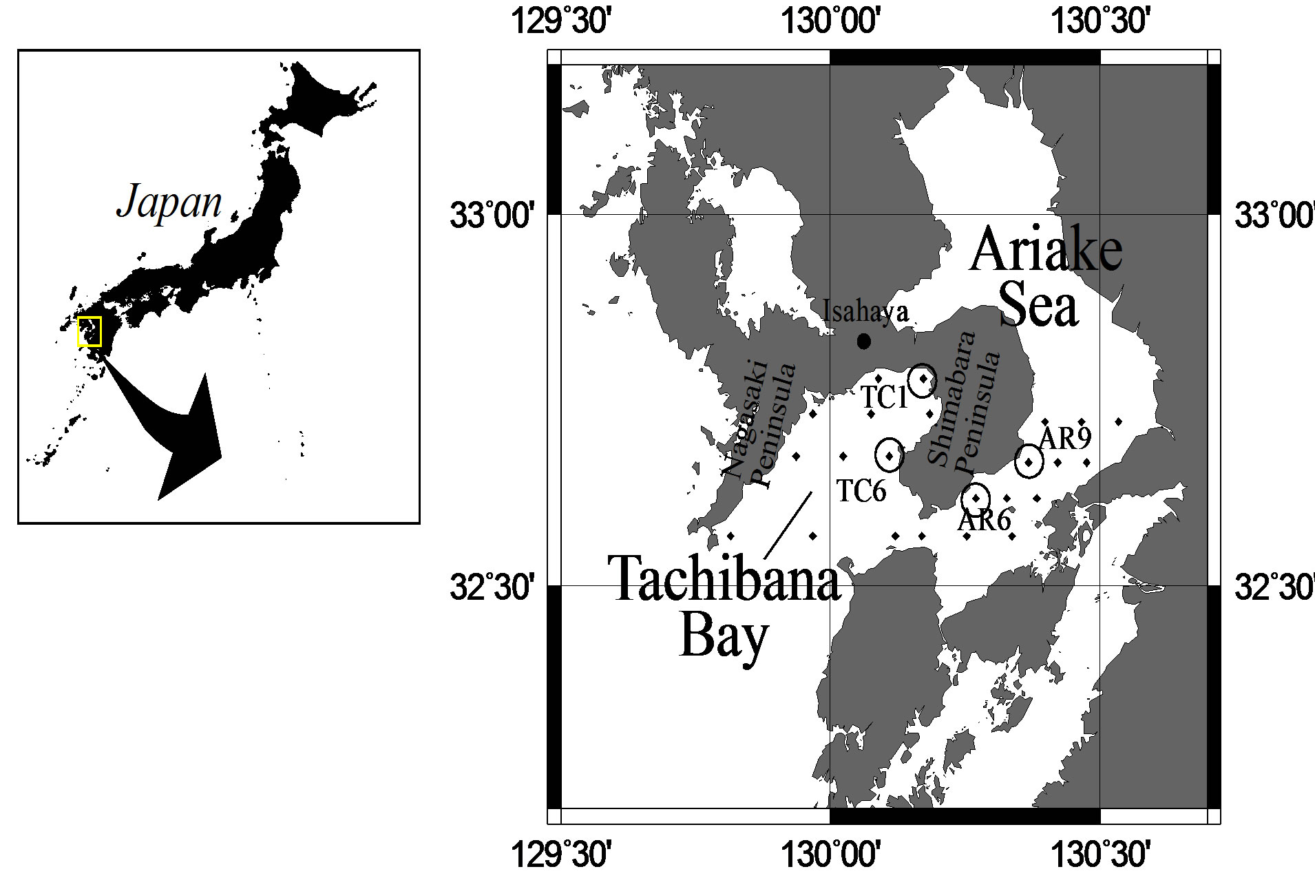
Figure 1. Study site map. A round mark shows a validation point. A point shows LCI matching point.
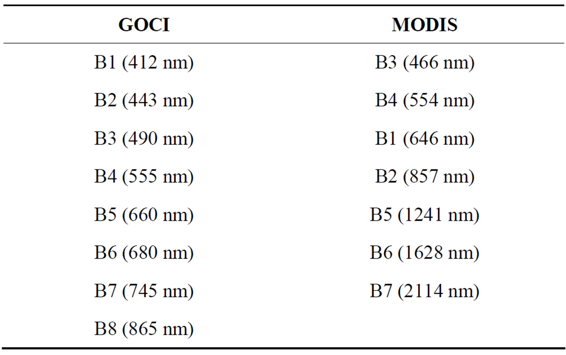
Table 1. Comparison between GOCI and MODIS bands.
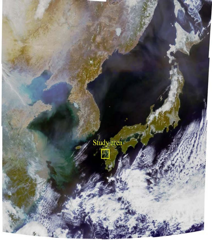
Figure 2. Example of a GOCI image and location of study area.
the sum of Ra (aerosol reflectance) and Rw (in-water reflectance). The LCI is the linear combination of two or more bands of Rtr given by
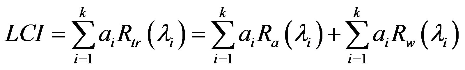 (1)
(1)
where 3 or 4 bands are usually combined, and the coefficient that accumulation of each band aiRa asked for ai in the meaning which removes the influence of atmospheric so that it might be exactly set to 0 here. Now, the LCI becomes the linear combination of the sea water reflectance of the 3 or 4 selected bands. In this way, atmospheric information is excluded, and only the water information is analyzed. Applying this LCI to three arbitrary bands (two visible and one near-infrared) of GOCI, we obtain the following LCI equation. The terms “nj = −1, 0.3”, which are used in calculations of 500-m resolution MODIS Chl.a data from JAXA, were used as coefficients expressing the type of aerosol in the present analysis.
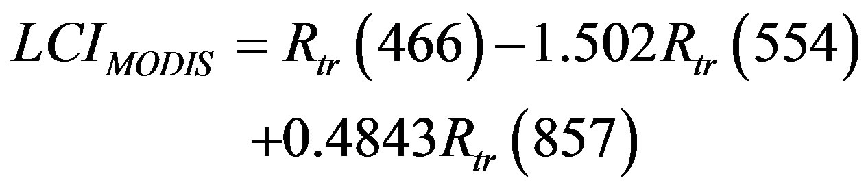 (2)
(2)
Applying the same approach to the GOCI data, the GOCI LCI is calculated as follows, theoretically.
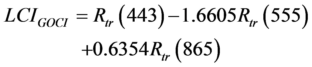 (3)
(3)
The calculated LCI is known to be closely related to Chl.a in the water area, i.e., phytoplankton concentration determines ocean color. The relationship between LCI and Chl.a along the Japanese coast can be modeled by:
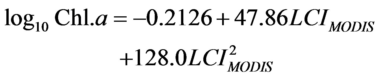 (4)
(4)
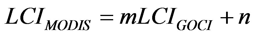
In this study, the MODIS Chl.a data are fused with the GOCI Chl.a data using Equations (2)-(4). First, MODIS LCI and GOCI LCI are assumed to be linearly related by
 (5)
(5)
where m and n are constants. GOCI LCI can be converted to MODIS LCI using Equation (5), then converted to Chl.a data from Equation (4).
2.4. Data Processing of GOCI and MODIS
First, GOCI Level 1B and MODIS LCI data were acquired from the KOSC and JAXA NRT websites. Next, the GOCI L1B data were converted to Rtr (L2) from the radiance (L1B) data using GDPS software ver.1.2.0. The Rtr data of GOCI at 443 nm (Band 2), 555 nm (Band 4), and 865 nm (Band 8) were used, as shown in Equation (3). These Rtr data were converted to GOCI LCI by Equation (2). The MODIS LCI and GOCI LCI were then compared at the LCI matching points indicated in Figure 1. A schematic of the GOCI Chl.a data processing and a list of GOCI/MODIS data sets for comparison between the LCIs are shown in Figure 3 and Table 2, respectively.
2.5. Validation Data Set
Chl.a calculated by the flowchart shown in Figure 3 was validated by comparison with in-situ Chl.a data acquired at sites TC1, TC6, AR6, and AR9 (Figure 1) on August 7 and 8, 2012, as shown in Table 3. The water sample was filtered by using a glass fiber filter (GF/F; Whatman Ltd.). The Chl.a was fluorometrically determined using a fluorometer (Turner Designs Inc.) after extracting the pigments in N,N-dimethylformamide (DMF). The GOCI data closest to the local observation time were also extracted for comparison (in the case of TC1, the GOCI data collected at the 2nd nearest time were selected because of cloud cover).
3. Results and Discussion
3.1. Comparison between GOCI and MODIS Linear Combination Index
The relationship between the GOCI and MODIS LCIs in
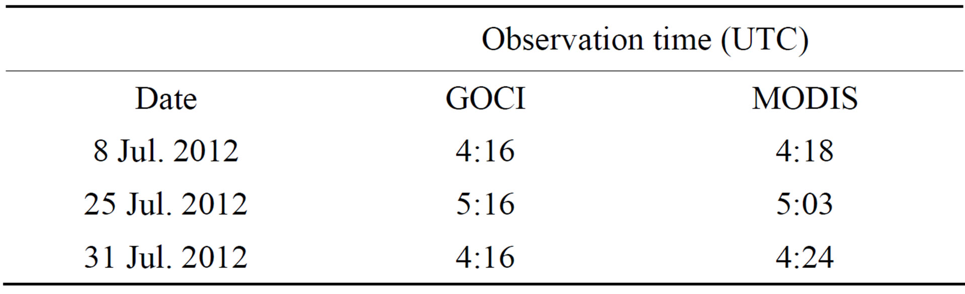
Table 2. List of GOCI/MODIS data set for comparison between GOCI and MODIS LCIs.
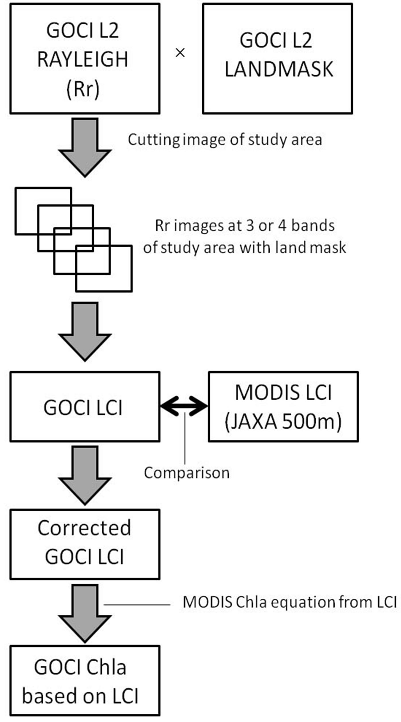
Figure 3. Schematic of data-processing process of GOCI Chl.a.
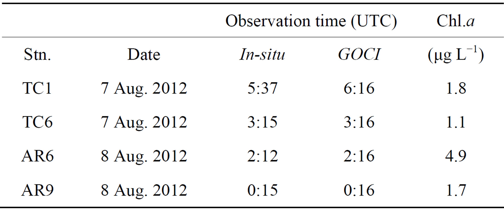
Table 3. List of in-situ Chl.a and GOCI data sets for the LCI algorithm.
Tachibana Bay, estimated from Equations (3) and (4), respectively, is shown in Figure 4. Significant correlation (R = 0.84) is observed, and the following conversion equation between GOCI LCI and MODIS LCI is obtained. GOCI LCI was converted to MODIS LCI from Equation (4) and then converted to Chl.a using Equation (5).
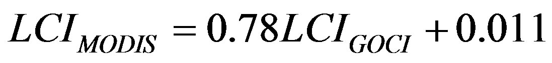 (6)
(6)
3.2. Validation of GOCI Chlorophyll-A
Figure 5 compares the Chl.a maps of MODIS and GOCI, derived from Equations (6) and (4). The maps are based on the data of June 10, 2012. The two maps show strong qualitative agreement.
To enable quantitative assessment of the GOCI Chl.a
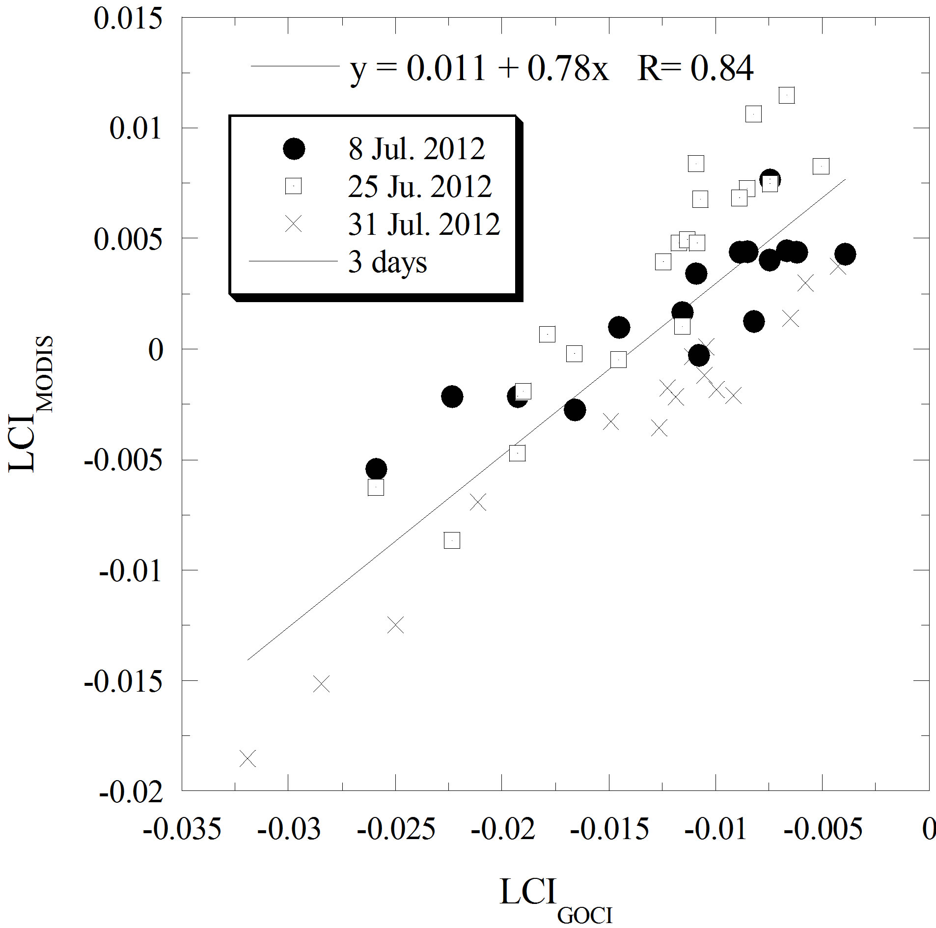
Figure 4. Relationship between GOCI LCI and MODIS LCI in Tachibana Bay, from data collected on July 8, July 25, and July 25, 2012.
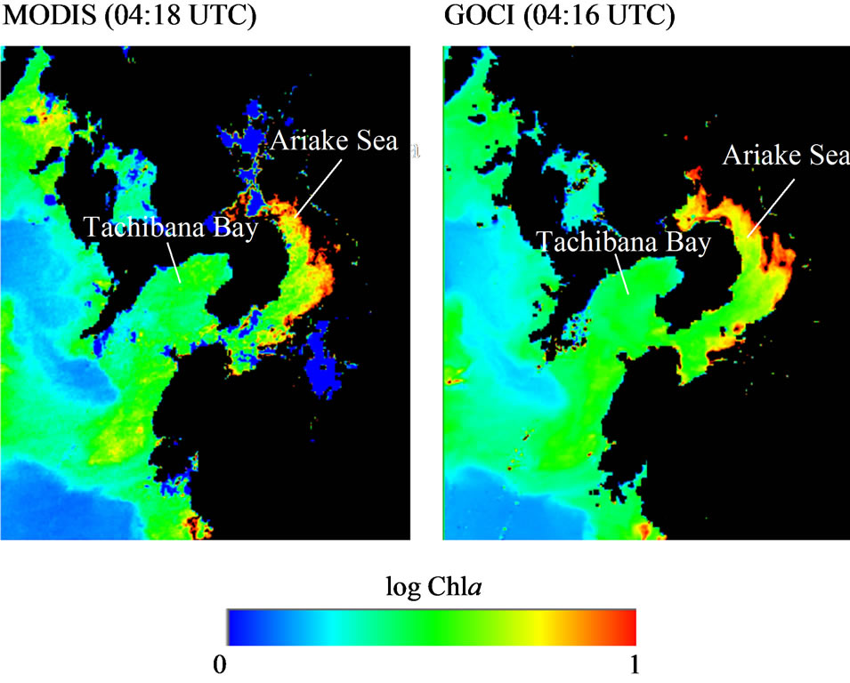
Figure 5. Comparison between MODIS Chl.a (left) and GOCI Chl.a (right), following LCI fusion of data collected on June 10, 2012.
concentration, the GOCI Chl.a (computed from Equations (6) and (4)) was plotted as a function of in-situ Chl.a. The relationship is shown in Figure 6. In this figure, the coincidence is high in Tachibana Bay, but poor in Ariake Sea, probably because the LCI algorithm is inaccurate in open seas (Case I) [7]. The optical characteristics of the sea water in the Ariake Sea might be altered by suspended matter, CDOM, and algal bloom [2,8]. Moreover, the initial Ariake Sea data were collected under filmy cloud, which may also have exerted an influence. To properly evaluate the cause of the discrepancy, a larger validation data set is required.
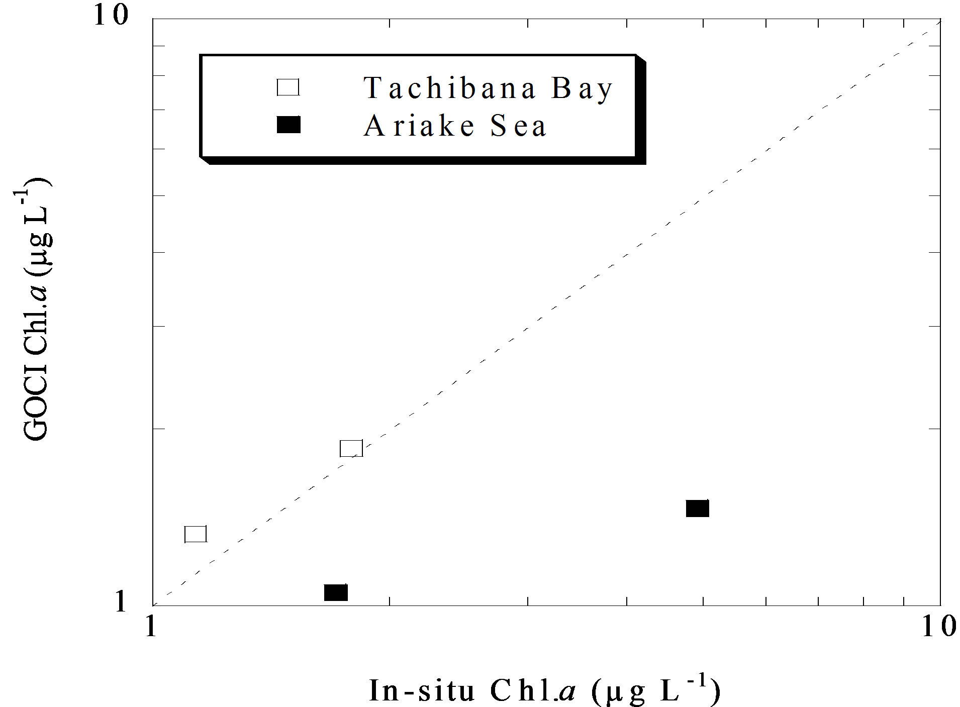
Figure 6. Relationship between in-situ Chl.a and GOCI Chl.a estimated from Equations (6) and (4) in Tachibana Bay on August 7 and August 8, 2012.
3.3. Temporal Feature of GOCI Chlorophyll-A Map
Figure 7 displays the GOCI Chl.a time series evaluated from Equations (6) and (4) from 00 h to 07 h UTC on 25 Jul. 2012. The Chl.a distribution pattern in Tachibana Bay markedly changes over time. Temporal changes in Chl.a concentration are particularly strong in the whirlpool region indicated by the arrow in Figure 7. This result is consistent with the pattern of strong streaming from Ariake Sea, which accompanies tidal flows to Tachiba Bay [9]. This is likely the first report in which a time migratory pattern of Chl.a interlocked with such flows has been examined by satellite imagery, and Figure 7 will become a very significant example.
4. Conclusions
This study has established a technique for converting MODIS to GOCI LCI. The achievements of the study are summarized below.
1) Adopting a JAXA MODIS LCI technique, a theoretical GOCI LCI equation was obtained.
2) The GOCI Chl.a was calculated from JAXA 500 m MODIS Chl.a using the GOCI Level2 Rayleigh product.
3) The LCI method yielded significant correlation between JAXA MODIS LCI and GOCI LCI.
4) GOCI Chl.a concentrations estimated by the proposed technique well agreed with in-situ Chl.a concentrations in Tachibana Bay.
Since the GOCI Level2 Rayleigh corrected reflectance product has been here demonstrated for the first time, the technique was evaluated on a very restrictive dataset. To properly validate the proposed method, evaluation on more extensive datasets is required, and it will be undertaken in our future study. Eventually, we hope to establish a Chl.a database system that will assist local fishery
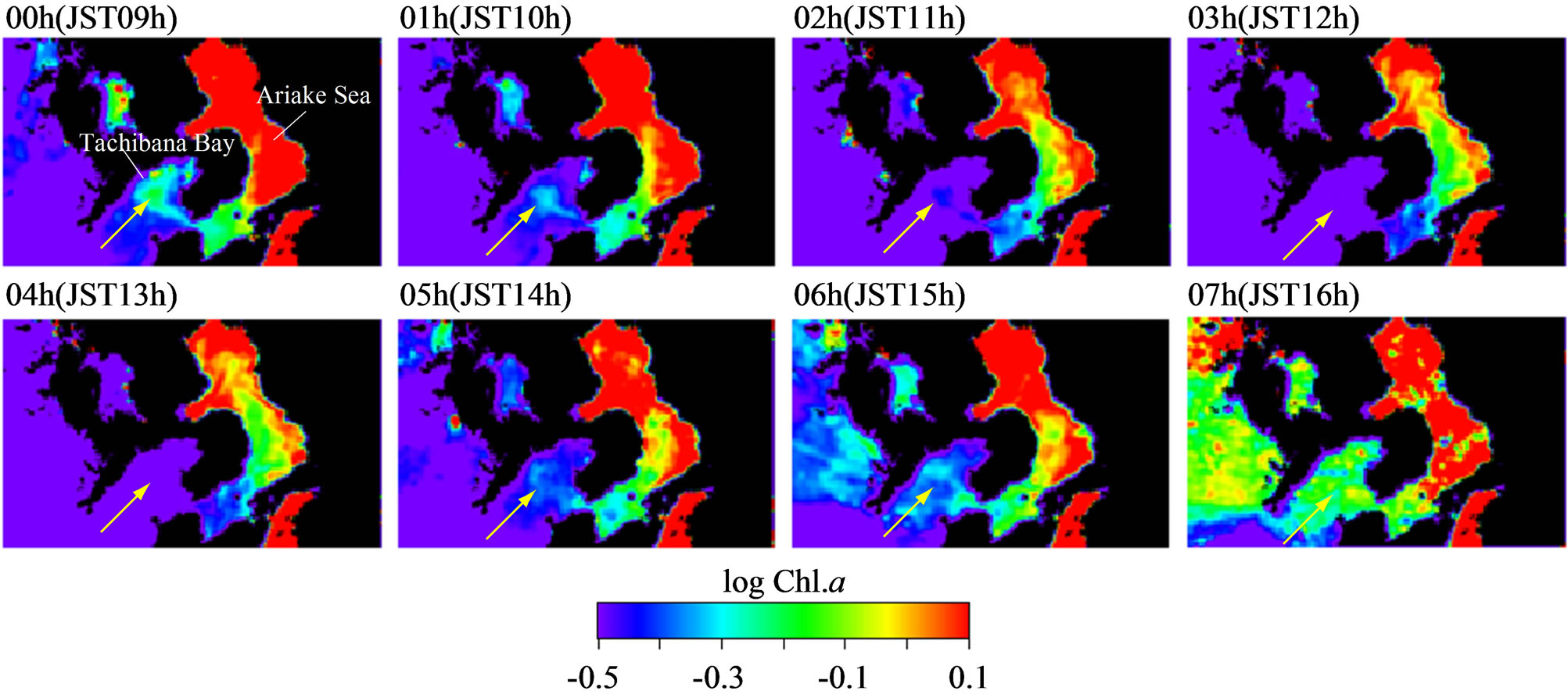
Figure 7. GOCI Chl.a time series from 00 h to 07 h UTC, 25 Jul. 2012 (Unit of scale bar: log Chl.a).
operators and other users of the bay.
5. Acknowledgements
GOCI data were provided by Korea Ocean Satellite Center/Korea Institute of Ocean Science & Technology and/ or this study was a part of the project titled “Support for research and applications of Geostationary Ocean Color Imager (GOCI)” funded by the Ministry of Land, Transport and Maritime Affairs, Korea. A part of this study was supported by the Japan Society for the Promotion of Science KAKENHI (23404001, 24404006, and 24560623).
REFERENCES
- K. Matsuoka, M. Iwataki and H. Kawami, “Morphology and Taxonomy of Chain-forming Species of the Genus Cochlodinium (Dinophyceae),” Harmful Algae, Vol. 7, No. 3, 2008, pp. 261-270. http://dx.doi.org/10.1016/j.hal.2007.12.002
- I. Imai, “Biology and Ecology of Chattonella Red Tides,” Seibutsu-Kenkyusha, Tokyo, 2012. (in Japanese)
- J. Ishizaka, et al., “Satellite Detection of Red Tide in Ariake Sound, 1998-2001,” Journal of Oceanography, Vol. 62, No. 1, 2006, pp. 37-45. http://dx.doi.org/10.1007/s10872-006-0030-1
- Japan Aerospace Exploration Agency, Earth Observation Research Center, “MODIS Near Real Time Data.” http://kuroshio.eorc.jaxa.jp/ADEOS/mod_nrt_new/index.html
- R. Frouin, P. Deschamps, L. Gross-Colzy, H. Murakami and T. Nakajima, “Retrieval of Chlorophyll-a Concentration via Linear Combination of ADEOS-II Global Imager data,” Journal of Oceanography, Vol. 62, No. 3, 2006, pp. 331-337. http://dx.doi.org/10.1007/s10872-006-0058-2
- J.-H. Ryu, H.-J. Han, S. Cho, Y.-J. Park and Y.-H. Ahn, “Overview of Geostationary Ocean Color Imager (GOCI) and GOCI Data Processing System (GDPS),” Ocean Science Journal, Vol. 47, No. 3, 2012, pp. 223-233.
- A. Morel and L. Prieur, “Analysis of Variations in Ocean Color,” Limnology and Oceanography, Vol. 22, No. 4, 1977, pp. 709-722. http://dx.doi.org/10.4319/lo.1977.22.4.0709
- H. Sasaki, et al., “Optical Properties of the Red Tide in Isahaya Bay, Southwestern Japan: Influence of Chlorophyll a Concentration,” Journal of Oceanography, Vol. 64, No. 4, 2008, pp. 511-523. http://dx.doi.org/10.1007/s10872-008-0043-z
- M. Tanaka, S. Inagaki and K. Yamaki, “Numerical Simulation of Tide and Three Dimensional Flow in Ariake Bay,” Proceedings of Coastal Engineering, JSCE, Vol. 49, 2002, pp. 406-410. (in Japanese) http://dx.doi.org/10.2208/proce1989.49.406