Advances in Remote Sensing
Vol.2 No.1(2013), Article ID:28965,6 pages DOI:10.4236/ars.2013.21002
Noise Reduction in White Light Lidar Signal Using a One-Dim and Two-Dim Daubechies Wavelet Shrinkage Method
1Institute for Laser Technology, Suita, Osaka, Japan
2Physics Department, De La Salle University, Manila, Philippines
3Department of Earth and Space Science, Osaka University, Osaka, Japan
Email: somekawat@ile.osaka-u.ac.jp, maria.cecilia.galvez@dlsu.edu.ph
Received November 7, 2012; revised December 25, 2012; accepted January 3, 2013
Keywords: White Light Lidar; Multi-Wavelength; Wavelet; Daubechies
ABSTRACT
A 1-D and 2-D Daubechies 5 (db5) discrete wavelet shrinkage methods using a 10 level decomposition was applied to white light lidar data particularly at 350 nm and 550 nm backscattered signal. At 350 nm, the backscattered signal is very weak as compared to 550 nm backscattered signal because of the spectral intensity distribution of the generated white light. The 1-D and 2-D wavelet shrinkage method gave a much better result as compared with the moving average method. However, the 2-D wavelet shrinkage method produced a much better denoised lidar signal compared with the 1-D wavelet shrinkage method. This is indicated by the 142% increase in correlation coefficient between the 2-D denoised lidar signal and the 800 nm original lidar signal as compared with only 12% increase in correlation coefficient for the 1-D denoised lidar signal. The 2-D wavelet shrinkage method also gave a much higher SNR value of 65.9 compared to 1-D which is 38.8.
1. Introduction
Supercontinuum generation on air and other gas media using high peak power femtosecond lasers opened the way for multispectral atmospheric remote sensing using a white light lidar. Because of its broad spectrum ranging from UV to IR, the technique offers several applications [1,2]. We have demonstrated that the coherent white light continuum can be used for depolarization and multiwavelength measurement in the same way as the conventional lidar [3]. However, multi-wavelength lidar observations for conventional lidar often use at least two laser sources. The multi-wavelength lidar measurements using a coherent white light continuum have the capability of obtaining the wavelength dependence of the backscatter coefficients of aerosols, which can be used to evaluate the particle size distribution using one laser source [1]. However, the present experiment does not fully utilize the potential of a broadband white light continuum. Lidar applications using the infrared region of the white light remains a challenge, because of the rapid decrease of the infrared content of the white light. Furthermore, the transmitted intensity of the white light was very weak for short wavelength (350 nm and 450 nm) as compared with the fundamental wavelength (800 nm). The signals are usually buried in noise, depending on the power of the laser and the observed altitude. In general, lidar signals with noise can be improved by moving average method. However, the moving average method only smoothen the signals and does not remove specky values especially the negative values produced by noises [4]. Lidar signals are often presented in single profile representing one acquisition (one dimension), or in terms of time-height-intensity (THI) display (two dimensions) to represent one observation period. In this paper, we propose a method to improve the lidar data by means of one dimensional (1-D) and two dimensional (2-D) wavelet shrinkage method since the wavelet function is of a localized property and has sensitivity to the transient signals such as lidar signal. In addition, since the WT has different resolutions on noise and signal, it can perform denoising process on lidar signal.
2. Denoising Algorithm
In our previous paper [5], we applied several wavelets to find the most suitable wavelet for white light lidar system described in [3]. These wavelets were Haar, Daubechies 2 (db2), 5 (db5), and 8 (db8), Symlets 2 (sym2), 5 (sym5), and 8 (sym8), and Coiflets 2 (coif2) and 5 (coif5). The result showed that db5 was the most suitable for our application, henceforth it is the one used for denoising the lidar signal discussed in this paper.
2.1. 1-D Wavelet Shrinkage
In the noise reduction based on WT, we have used the discrete WT (DWT) over the continuous WT (CWT) because CWT is often redundant and computationally expensive. The DWT involves transforming a given signal with wavelet basis functions by dilating and translating it in discrete steps [6].
The wavelet shrinkage [7] is a signal denoising technique based on the idea of thresholding the wavelet coefficients. The wavelet shrinkage method is shown in Figure 1 and can be summarized as follows:
1) Apply the DWT to the signal.
2) Estimate a threshold value.
3) Remove the coefficients that are smaller than the threshold.
4) Perform an inverse DWT and reconstruct the signal.
An algorithm for calculating discrete wavelet decom-
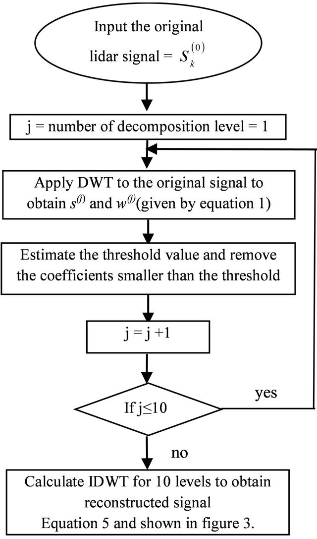
Figure 1. Flowchart of 1-D wavelet shrinkage method.
ositions and reconstructions is the Mallat algorithm [8].
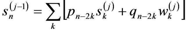
The noisy experimental signal f(t) is considered as , called a “scaling coefficient” at the 0 level of signal decomposition. Then, as shown in Figure 2, s(j) is successively decomposed into both s(j-1) and w(j-1) by the following formulas:
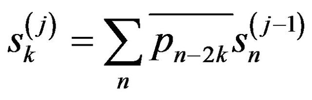 and
and 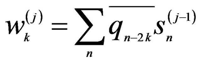 (1)
(1)
where w(j) is called the DWT coefficient, {pn} and {qn} are the sequence of coefficient.
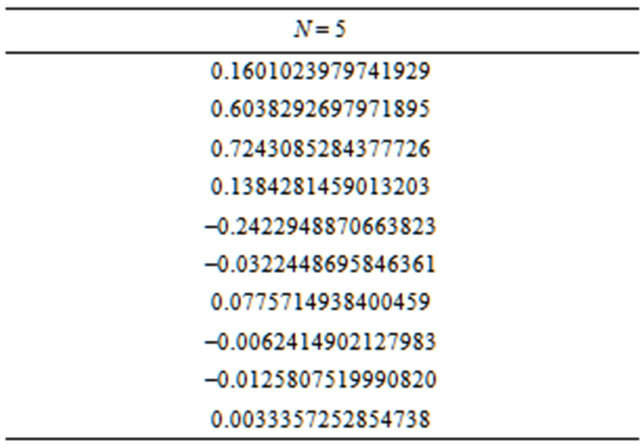
The sequences pn of Daubechies’ wavelet is given in Table 1 where qn is given by
 (2)
(2)
The level of noise in lidar data is unknown and must be estimated from the noisy data. In this algorithm we have used the universal threshold as suggested in [9],
 (3)
(3)
where N is the dimensionality of the input data vector and σ is the standard deviation of the noise. The σ is often estimated from the median value of the DWT coefficients at the first level of signal decomposition [4],
 (4)
(4)
Once the threshold value has been calculated, we can apply a soft threshold to reduce the noise in signal. If the magnitudes of the DWT coefficients, wk(j), are smaller than this threshold value, the DWT coefficients are replaced by zero, while the rest of them are calculated as wk(j) - T. Signal reconstruction can be presented as follows:
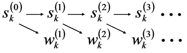
Figure 2. 1-D wavelet decomposition.
Table 1. Daubechies 5 wavelet sequence Daubechies compactly supported wavelet for N = 5.
 (5)
(5)
The denoised signal s(j-1) can be successively obtained from w(j) and s(j) as shown in Figure 3.
2.2. 2-D Wavelet Shrinkage
Figure 4 gives the flowchart for the 2-D wavelet shrinkage method (2-D). As shown in Figure 4, the noisy experimental image which is represented by the time-height-intensity (THI) display of the lidar signal is considered as  in the same way as 1-D wavelet shrinkage (1-D). DWT is applied first to
  in the horizontal direction, represented by the time component of the lidar return signal. The coefficients applied in the
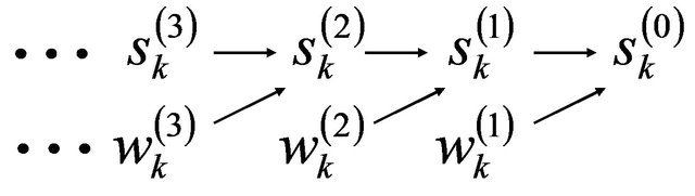
Figure 3. 1-D wavelet reconstruction.
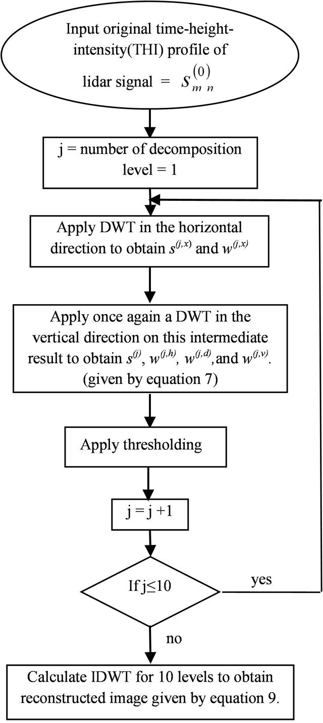
Figure 4. Flowchart of 2-D wavelet shrinkage method.
horizontal direction of the scaling function (sm,n(j+1,x)) and the wavelet function (wm,n(j+1,x)) are given by
 (6a)
(6a)
 (6b)
(6b)
Secondly, DWT is also applied in the vertical direction to the obtained coefficients, and these are given by:
 (7a)
(7a)
 (7b)
(7b)
 (7c)
(7c)
 (7d)
(7d)
where  is the coefficient which is applied to the scaling function in the horizontal direction and to the wavelet function in the vertical direction;
  is the coefficient which is applied to the wavelet function in the horizontal direction and to the scaling function in the vertical direction; and
  is the coefficient which is applied to the wavelet function in both directions. The vertical direction represents the height component of the lidar return signal.
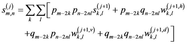
Then, the algorithm for the computation of the  can be summarized by the following four equations:
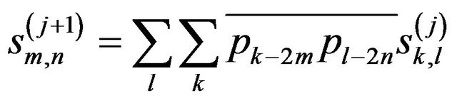 (8a)
(8a)
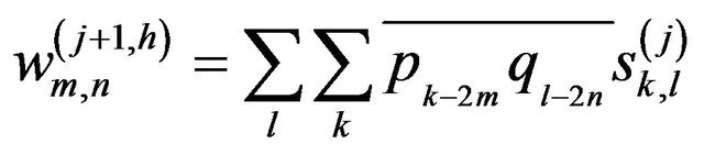 (8b)
(8b)
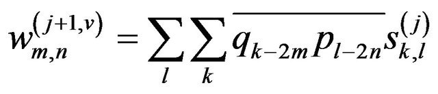 (8c)
(8c)
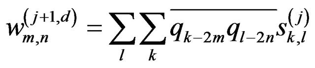 (8d)
(8d)
The same procedure is done for  and successively decomposed
  in 2-D. Finally, the de-noised image can be reconstructed by
 (9)
(9)
Figure 5 shows an example of one level decomposition 2-D wavelet transform.
3. Experimental Results and Discussion
In this section, we apply the 1-D and 2-D wavelet de-
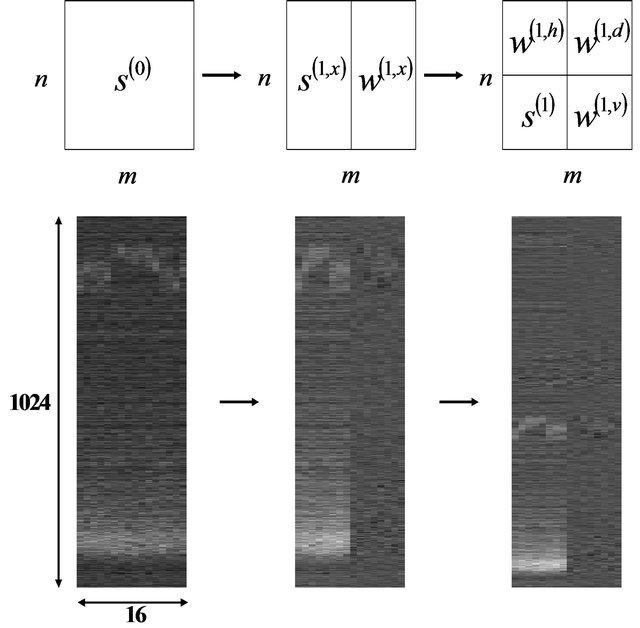
Figure 5. One level decomposition 2-D wavelet transform.
noising algorithms for reducing noise in previous observational results found in [3]. We have taken a data size of 1024 (= 210) points and decomposed into 10 levels for 1-D and 2-D wavelet denoising.
3.1. 1-D wavelet Signal Denoising
Figure 6 shows the denoised lidar signal based on the above 1-D denoising procedure with soft threshold. For comparison, the real signal and moving average signal are presented in Figure 6. In order to check whether our method can filter the noise out and also extract the cloud signals, the channel with the weakest backscattered signal, 350 nm, is compared to the channel which relatively has strong backscattered signal, 550 nm. Figure 6(a) shows the backscattered signal at 550 nm. Cloud peaks can be seen at about 0.5 km and 1 km. For the strong 550 nm backscattered signals, the 1-D wavelet denoising method applied to the signal caused no significant difference. However, it can be found that cloud signals which were buried in noise in the weaker channel at 350 nm became noticeable after the denoising procedure by comparing Figure 6(b) with Figure 6(a). Thus, this method can effectively detect the lidar signal buried in noise and thus reduce the noise.
3.2. 2-D Wavelet Signal Denoising
The 2-D wavelet signal denoising technique was applied to time height intensity (THI) display to evaluate the performance of the proposed 2-D method. Since the backscattered lidar signals diminish with the square of the range, the signals were corrected accordingly. This improved to a considerable degree the visualization and interpretation of the obtained lidar signals. The matrix
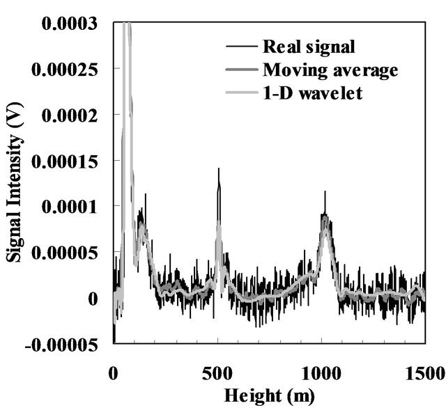 (a)
(a)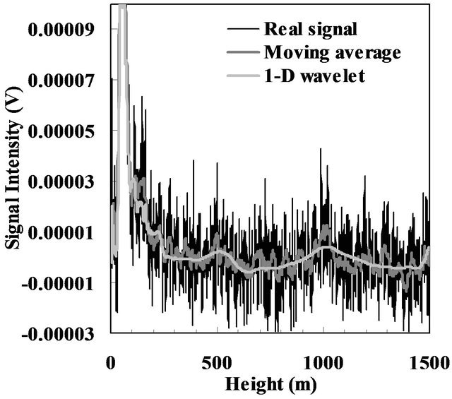 (b)
(b)
Figure 6. The original lidar signal from (a) 550 nm and (b) 350 nm and the corresponding denoised lidar signals using moving average and 1-D wavelet shrinkage (2005/03/23 2:13).
size of the reconstructed THI image is 1024 × 1024. We assume that the horizontal length of the stored signal dataset is extended to 1024 by repeating the 16-min data set. The moving average for range series improves the signal-to-noise ratio and the image quality of experimental lidar THI image especially at 550 nm. But the result of this method still includes the noise. In the moving average THI image at 350 nm, it is not easy to discriminate the high-altitude cloud structures because the noise are generally more pronounced at higher altitude. As shown in Figure 7(a), the 1-D db5 wavelet denoised images gave improved results. However, the 1-D wavelet denoised images become discontinuous in the horizontal direction because it was applied solely to the intensity level on the vertical line. Lower cloud layers vary more rapidly as compared to higher altitude clouds during the observation. This can be clearly seen in Figure 8. In Figure 8, the original 800 nm lidar signal is shown together with the original 350 nm lidar signal and the denoised 350 nm lidar signal using the 1-D and 2-D wavelet shrinkage method. At 2:11 am, the 800 nm lidar signal showed two layers of clouds, one just above 500 m and the other one near 1000 m. However this was not
 (a)
(a)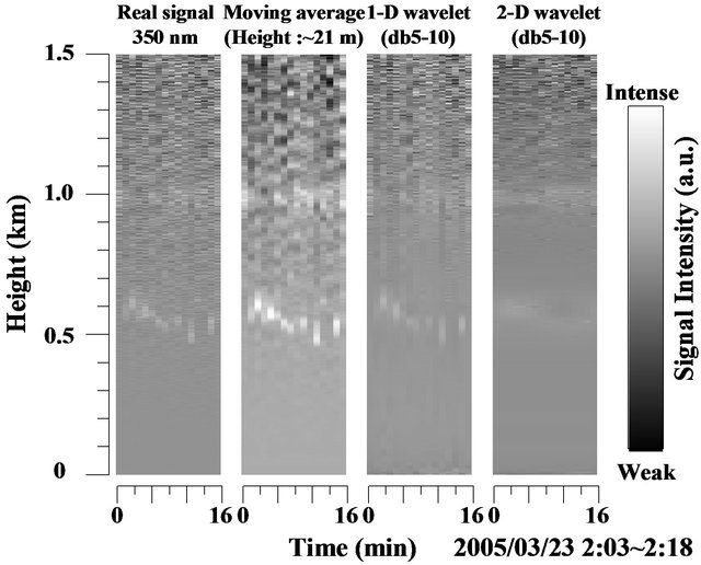 (b)
(b)
Figure 7. The original lidar image from (a) 550 nm and (b) 350 nm and the corresponding denoised lidar images using moving average, 1-D wavelet shrinkage, and 2-D wavelet shrinkage.
seen on the 350 nm lidar signal. Application of the 1-D wavelet shrinkage method on the 350 nm lidar signal revealed the second cloud layer but not the lower cloud layer as shown in Figure 8(a). This explains the discontinuity in the lower cloud layer detection for the 1-D wavelet shrinkage method. But using the 2-D wavelet shrinkage method on the same 350 nm lidar signal, the two cloud layers were revealed, as shown in Figure 8(b). In 2-D wavelet denoising, we perform additional horizontal smoothing. We also calculated the correlation coefficient of the 800 nm lidar signal with the 350 nm original lidar signal, 1-D wavelet, and 2-D wavelet denoised signal. The correlation coefficient was applied only on the higher cloud layer which is about 1000 m to determine the degree of similarity of the shape of the cloud signal. The correlation coefficients are 0.27, 0.31, and 0.67 for the original, 1-D denoised, and 2-D denoised 350 nm lidar signals, respectively. In terms of percent increase in correlation of the 350 nm signal with the 800 nm signal, a 12% increase in correlation was observed for the 1-D and a 146% increase in correlation
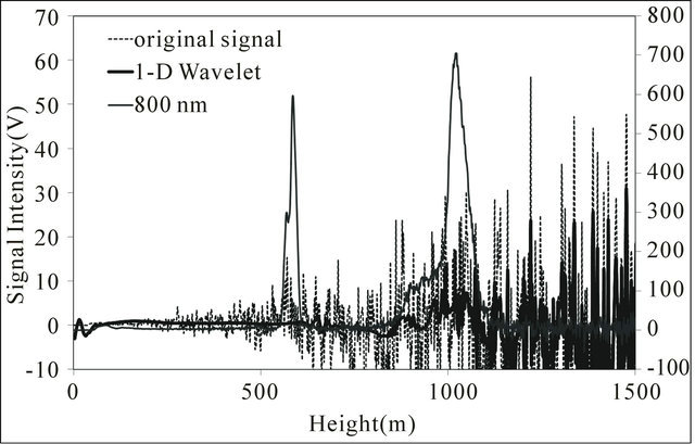 (a)
(a)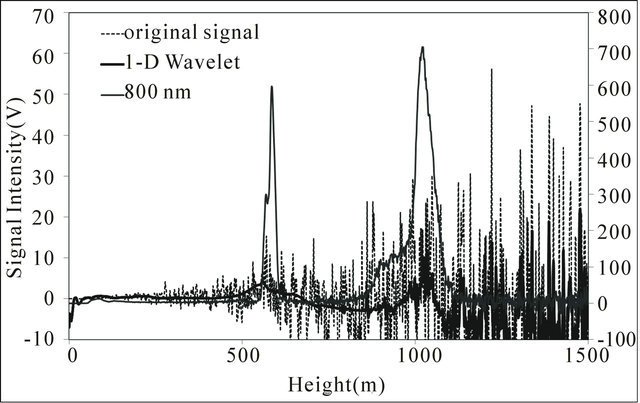 (b)
(b)
Figure 8. The original lidar signal from 800 nm and 350 nm and the corresponding denoised lidar signals for 350 nm using (a) 1-D and (b) 2-D wavelet shrinkage (2005/03/23 2:11).
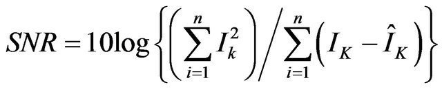
was observed for the 2-D. It is also noticeable in Figure 8 that the shape of the higher cloud layer for 350 nm 2-D wavelet denoised signal shows similarity with the 800 nm as compared with the 1-D wavelet denoised signal. We also evaluated the signal-to-noise ratio (SNR) using [4]
 (10)
(10)
where  and
and  denotes denoised signal and the original signal, respectively. The calculated SNR were 38.8 and 65.9 for 1-D and 2-D wavelet method, respectively.
4. Conclusion
1-D and 2-D wavelet denoising were applied to white light lidar signals using Daubechies 5 level 10. Although the wavelet denoising methods cause no significant improvement for strong backscattered signals at 550 nm, they are effective in extracting the signals from the noisy experimental data for the weaker channel at 350 nm. Compared with other methods such as the moving average method, the 1-D and 2-D wavelet shrinkage are better in reducing the noise. Evaluation of the the 1-D and 2-D wavelet shrinkage method showed that the 2-D method was better in revealing the signals buried in noise such as the dynamic lower cloud layer as indicated by the higher SNR of 2-D compared with 1-D and a higher correlation coefficient of the 2-D with the original 800 nm lidar signal. However, the shape of the lower cloud layer signal as compared with the lidar signal from strong channels such as the 800 nm was not really comparable although it was able to reveal the presence of the cloud at that height. The 1-D wavelet shrinkage method was not able to reveal the abovementioned cloud layer. For the higher altitude cloud layer which was quite stable during the whole observation, the 2-D wavelet shrinkage method also gave a much better improved cloud profile. Wavelet denoising is often inadequate for the rapid changes in cloud at low altitude when attempting to separate signals from noisy data but for high-altitude clouds, the obtained cloud profiles are slightly improved. This seems to be the key feature in 2-D wavelet denoising as compared with the moving average or 1-D wavelet denoising. With the 2-D wavelet denoising method, signal detection from IR to UV using the white light lidar signal is possible especially if there are no rapid changes in the cloud layer or aerosol and any lidar signal for that matter. This will allow us to retrieve the microphysical properties of cloud or aerosol layers, such as particle size. However, faster data acquisition is necessary to be able to capture the rapid changes in the aerosol or cloud layers.
REFERENCES
- M. C. D. Galvez, et al., “Three-Wavelength Backscatter Measurement of Clouds and Aerosols Using a White Light Lidar System,” Japanese Journal of Applied Physics, Vol. 41, No. 3, 2002, pp. L284-L286. doi:10.1143/JJAP.41.L284
- P. Rairoux, et al., “Remote Sensing of the Atmosphere Using Ultrashort Laser Pulses,” Applied Physics B, Vol. 71, No. 4, 2000, pp. 573-580. doi:10.1007/s003400000375
- T. Somekawa, M. Fujita, C. Yamanaka and M. C. D. Galvez, “Depolarization Light Detection and Ranging Using a White Light LIDAR System,” Japanese Journal of Applied Physics, Vol. 45, No. 6, 2006, pp. L165-L168. doi:10.1143/JJAP.45.L165
- H. T. Fang and D. S. Huang, “Noise Reduction in Lidar Signal Based on Discrete Wavelet Transform,” Optics Communications, Vol. 233, No. 1-3, 2004, pp. 67-76. doi:10.1016/j.optcom.2004.01.017
- M. C. D. Galvez, T. Somekawa, C. Yamanaka and M. Fujita, “Wavelet Denoising Applied to Multiwavelength Depolarization White Light Lidar Measurement,” Proceedings of the 23rd International Laser Radar Conference, Nara, 24-28 July 2006, pp. 275-278.
- I. Daubechies, “Ten Lectures on Wavelets,” Society for Industrial and Applied Mathematics, Philadelphia, 1992. doi:10.1137/1.9781611970104
- D. L. Donoho, “De-Noising by Soft-Thresholding,” IEEE Transactions on Information Theory, Vol. 41, No. 3, 1995, pp. 613-627. doi:10.1109/18.382009
- S. Mallat, “A Theory for Multiresolution Signal Decomposition: The Wavelet Representation,” IEEE Transactions on Pattern Analysis and Machine Intelligence, Vol. 11, No. 7, 1989, pp. 674-693. doi:10.1109/34.192463
- B. Walczak and L. Massart, “Noise Suppression and Signal Compression Using the Wavelet Packet Transform,” Chemometrics and Intelligent Laboratory Systems, Vol. 36, No. 2, 1998, pp. 81-94. doi:10.1016/S0169-7439(96)00077-9