American Journal of Plant Sciences
Vol.4 No.8(2013), Article ID:35336,8 pages DOI:10.4236/ajps.2013.48187
Determination of Energetic and Geometric Properties of Plant Roots Specific Surface from Adsorption/Desorption Ishoterm
![]()
Institute of Agrophysics of Polish Academy of Sciences, Lublin, Poland.
Email: *jozefaci@demeter.ipan.lublin.pl
Copyright © 2013 Grzegorz Jozefaciuk et al. This is an open access article distributed under the Creative Commons Attribution License, which permits unrestricted use, distribution, and reproduction in any medium, provided the original work is properly cited.
Received April 29th, 2013; revised May 31st, 2013; accepted June 15th, 2013
Keywords: Adsorption Energy; Adsorption/Desorption Isotherm; Fractal Dimension; Nanopore; Plant Roots
ABSTRACT
Background and Aims: Structure and composition of plant roots surfaces are extremely complicated. Water vapor adsorption/desorption isotherm is a powerful tool to characterize such surfaces. The aim of this paper is to present theoretical approach for calculating roots surface parameters as adsorption energy, distribution of surface adsorption centers, as well as roots geometric and structure parameters as surface fractal dimension, nanopore sizes and size distributions on example of experimental isotherms of roots of barley taken from the literature. This approach was up to date practically not applied to study plant roots. Methods: Simplest tools of theoretical analysis of adsorption/desorption isotherms are applied. Results: Parameters characterizing energy of water binding, surface complexity and nanopore system of the studied roots were calculated and compared to these of the soils. Some possible applications of root surface parameters to study plant-soil interactions are outlined. Conclusions: Physicochemical surface parameters may be important for characterizing root surface properties, their changes in stress conditions, as well as for study and model plant processes. Physicochemical and geometrical properties of plant roots differ from these of the soils.
1. Introduction
Surfaces natural adsorbents including plant roots are very complicated from chemical and structural points of view. To characterize such surfaces the adsorption/desorption isotherm of a gas or vapor is a very powerful tool, providing information on the surface area, adsorption energy, distribution of surface adsorbing centers, volume, radii and size distribution of nanopores, and surface fractal dimension. These surface parameters are not only used to describe surface properties, but also to evaluate and model many processes occurring in solid/ liquid or solid/gas interfaces, including soils, clays, clay minerals, industrial adsorbents and catalysts, chromatographic beds, and others, however they have been very rarely used to study plant materials. Application of adsorption isotherms to determine the area of plant roots specific surface was described in [1]. The present paper is designed to present theoretical aspects of calculation of plant roots surface properties basing on adsorption/desorption isotherms taken from the above cited paper.
2. Materials
Water vapor adsorption/desorption isotherms on air dried, 105˚C dried and lyophilized whole and cut roots of barley Hordeum (Ars) Stratus grown in hydroponic cultures, measured using vacuum chamber method were used. The detailed description of the experimental material and of the adsorption/desorption isotherms measurements can be found in [1] where from the isotherms considered in the present paper are redrawn into Figures 1 and 2.
3. Interpretation of the Isotherm
The S-shape of the isotherms indicates that the adsorption has polymolecular character as it occurs on most natural adsorbents, including plant roots. There are a few equations describing polymolecular adsorption isotherm, among which the Brunauer-Emmett-Teller model [2] is considered a standard. However, due to its thermodynamic incorrectness we apply very similar, Aranovich [3]
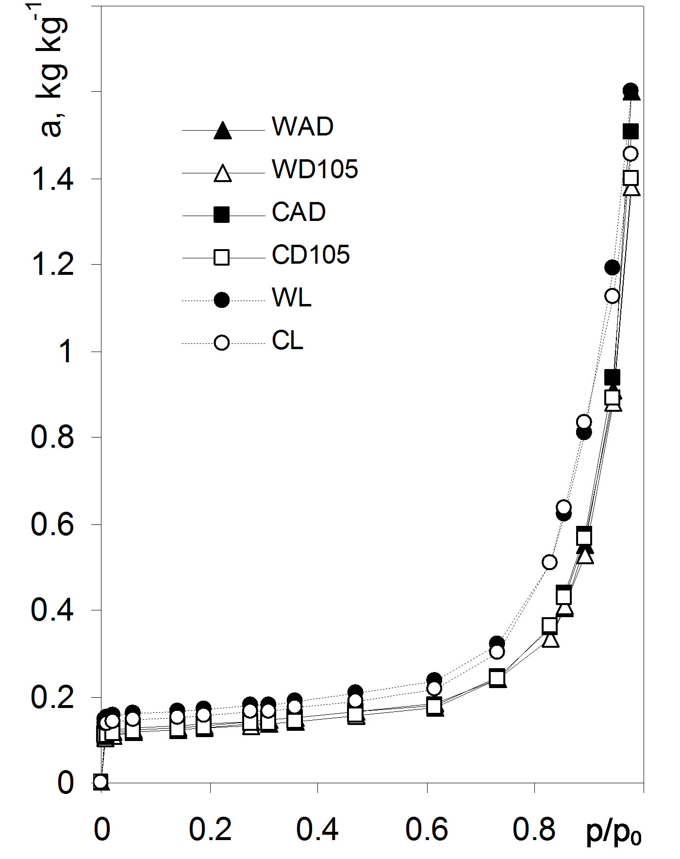
Figure 1. Water vapor adsorption isotherms on variously pretreated barley roots. Abbreviations for the pretreatments: WAD—whole roots air dried, WD105—whole roots dried at 105˚C, CAD—cut roots air dried, CD105—cut roots dried at 105˚C, WL—whole roots lyophilized, CL— cut roots lyophilized. The isotherms show average data from 9 isotherms (3 independent adsorption/desorption runs for 3 replicates each). Source: [1].
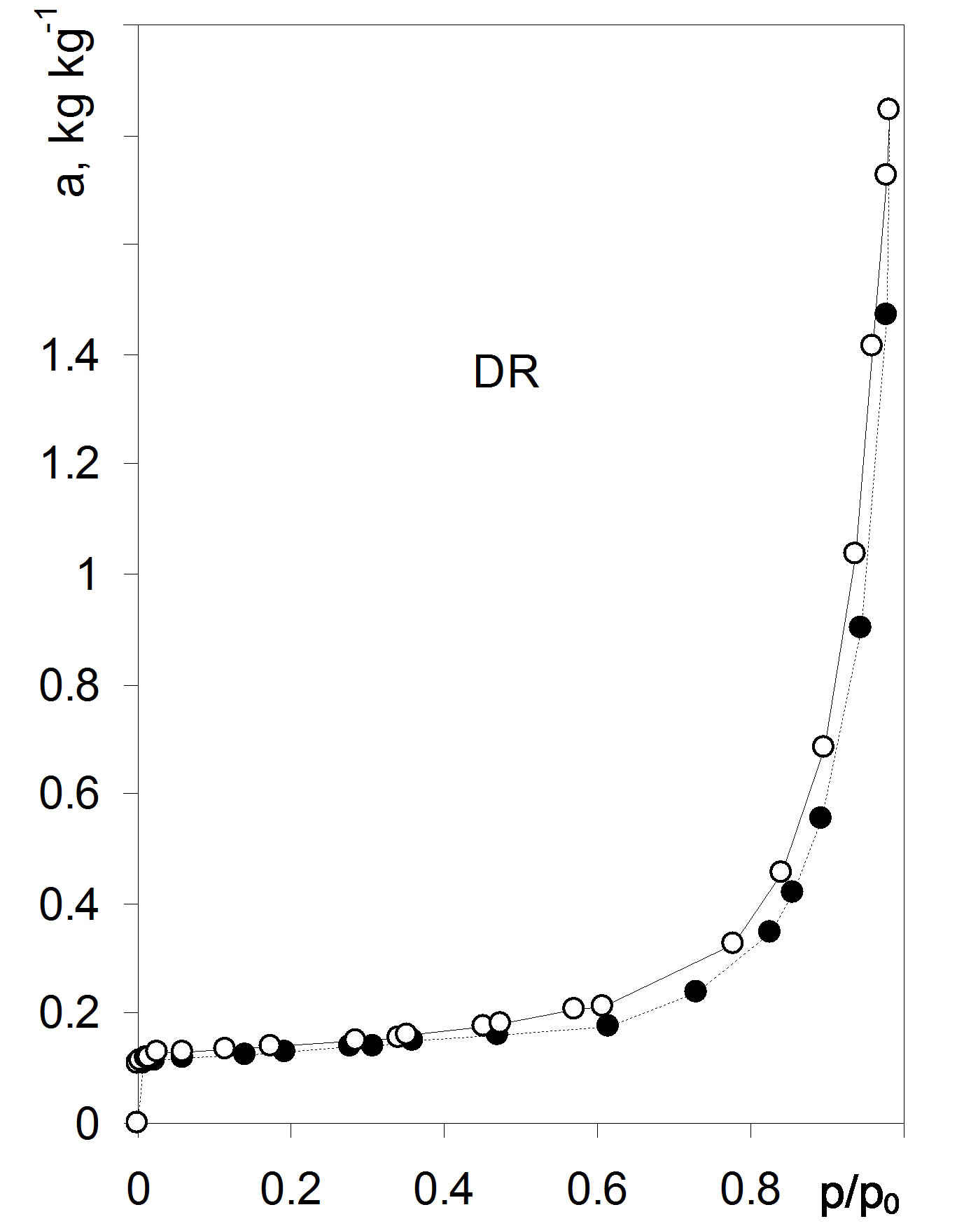
Figure 2. Adsorption/desorption isotherms for the barley roots. Dashed line: adsorption, solid line: desorption. The curves are average isotherms for whole, cut, air dried and 105˚C dried roots. Data are average from 36 isotherms. Source: [1].
equation, which reads:
 (1)
(1)
where a [kg·kg−1] is the amount of the adsorbed vapor at the relative vapor pressure p/p0 and at the temperature T [K], am [kg·kg−1] is a monolayer capacity, C = exp((Ea − Ec)/RT) is a constant related to the adsorption energy, Ea [J·mol−1], and the condensation energy of water, Ec [J·mol−1], and R [J·mol−1·K−1] is the universal gas constant.
A few mechanisms of adsorption can be distinguished in the whole range of relative vapor pressures. At low relative pressures, adsorption occurs mostly just near the surface, in the first adsorption layer (monomolecular adsorption), next the adsorbate molecules locate on the already adsorbed ones forming subsequent adsorption layers (polymolecular adsorption) and at relatively high relative pressures, the adsorbate vapor tends to condense in the adsorbent pores.
Different models can be applied to describe the above adsorption mechanisms that are usually not applicable in the whole range of relative adsorbate pressures. Using these models some important physicochemical characteristics of the adsorbent surface can be estimated: surface area, adsorption energy, distribution of surface adsorbing centers, fractal dimension, nanopore sizes and pore size distribution.
3.1. Adsorption Energy and Distribution of Surface Adsorbing Centers
Chemically different groups of atoms of various kind and polarity (e.g. carboxylic, hydroxylic, phosphate, amine, peptide, aliphatic and/or aromatic chains and radicals each located on various cell components: walls, membranes, protoplasts, nucleic acids, phospholipids, etc.) are present on root surfaces. These different surface groups (adsorption sites) bind adsorbate molecules with different forces (and energies) what in turn influence the adsorption pathways. The input of different energy sites to the total adsorption can be characterized by the adsorption energy distribution function. This function should be estimated from adsorption in the first layer (monolayer), because in next layers the surface adsorption forces are screened by already adsorbed molecules. Various models are used in the literature to find adsorption energy distribution function [4-6]. Here the simplest approach based on graphical (or numerical) differentiation of the adsorption in monolayer vs. adsorption energy curve, similarly as this is described in [7] is presented.
At first, one has to distinguish which part of the adsorbate locates in the monolayer. Knowing that the well known Langmuir equation describes monomolecular adsorption [8], to distinguish the monolayer region from polymolecular adsorption the Aranovich equation should be transformed to a form of a Langmuir-like one. The Langmuir equation is written as:
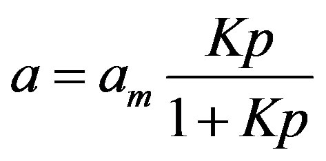 (2)
(2)
where K is a constant. A simple rearrangement of Equatio (2) gives:
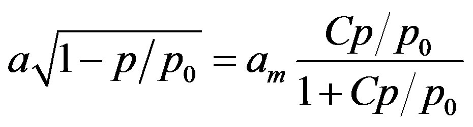 (3)
(3)
thus polymolecular adsorption a scaled by the factor (1 − p/p0)1/2 holds for adsorption in monolayer. Because the RHS of Equation (3) approaches am at high p/p0 values, alternatively to Equation (1), the monolayer capacity can be approximates as:
 (4)
(4)
Figure 3 shows adsorption in monolayer calculated applying Equation (3) for Figure 1 isotherms along with their monolayer capacities found using Equation (4). The values of a(1 − p/p0)1/2 calculated for high p/p0 range markedly exceed monolayer capacity values (calculated from Equations (4) and (1)). This reflects contribution of other mechanisms (e.g. capillary condensation) to polymolecular adsorption a, thus to find monolayer adsorption picture these points should be rejected (black points in Figure 3).
The empty points in Figure 3, lower than the preceding points, indicate that at the respective pressures no input to monolayer adsorption take place and only adsorption in the next layers occurs. These points are not
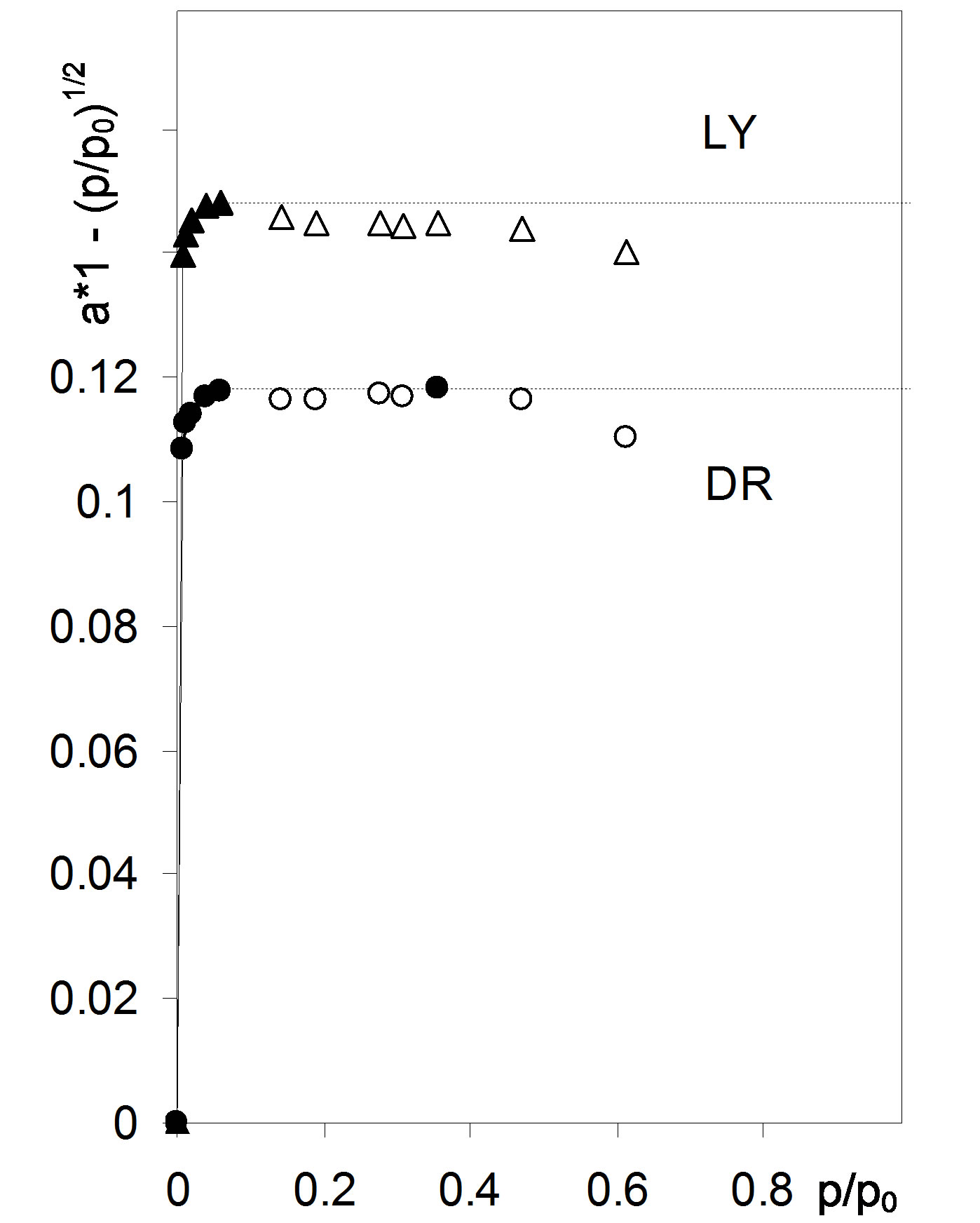
Figure 3. Monolayer adsorption for the studied root samples. The respective monolayer capacities calculated from Equation (4) are marked with dashed lines. Abbreviations DR: average data from 36 isotherms for whole, cut, air dried and 105˚C dried roots, LY: average data from 18 isotherms for whole and cut lyophilized roots.
considered in further estimation of energy distribution functions.
Because at the equilibrium the free energy is constant throughout the system, the energy of water vapor at a given relative pressure, RTln(p/p0), can be associated with adsorption energy. This is done using a formula:
 (5)
(5)
Adsorption energies are usually expressed as dimensionless energies showing an excess of adsorption energy over condensation energy of adsorbate in the units of RT (LHS of Equation (5) divided by RT). Dimensionless energies may be thus converted to adsorption energies: Ea [kJ·mol−1] = −44 + 2.48ln(p/p0), where −44 kJ·mol−1 is the condensation energy of water vapor and 2.48 kJ·mol−1 = RT for T = 298 K. The dimensionless energy equal to 0 holds for adsorption energy equal to the condensation energy of the adsorbate vapor that occurs at saturated vapor pressure (p0/p0 = 1 and ln(1) = 0), however at p0/p0 = 0 infinite adsorption energy is calculated (ln(0) = −∞). To avoid infinities, the maximum adsorption energy should be defined that should relate to the minimum value of the p0/p0 applied in the experiment. However, this value can be considered only as a first estimate of the maximum energy, because of the lack of experimental data at lower then minimum relative pres sures. Therefore somewhat higher maximum energy is selected arbitrarily. Because minimum p0/p0 value for the studied adsorption isotherms was 0.09 that corresponds to (Ea − Ec)/RT = −4.71 the maximum (Ea − Ec)/RT = −6 was set arbitrarily. Now one can construct a plot showing the amount of the adsorbate adsorbed in a monolayer versus (Ea − Ec)/RT, that is shown in Figure 4 (points not contributing to monolayer adsorption-empty points from Figure 3 are not included).
The dependence shown in Figure 4 serves for estimation of distribution function of surface adsorption centers. It can be assumed that the amount of adsorption on a given center of defined energy value is directly related to the number of adsorbing sites present on this center (one site adsorbs one adsorbate molecule). Thus the amount of adsorption on the centers kind i, ni [kg·kg−1] having energies ranging between Ei and Ei + ΔE, can be calculated as a value of a(Ei + ΔE) minus a(Ei) and the fraction of given energy centers in the whole adsorbent surface is given by:
 (6)
(6)
where Ei,av is the average adsorption energy of the center equal to (Ei + Ei + ΔE)/2.
So the distribution of surface adsorption centers is found by division of the adsorption energy range on
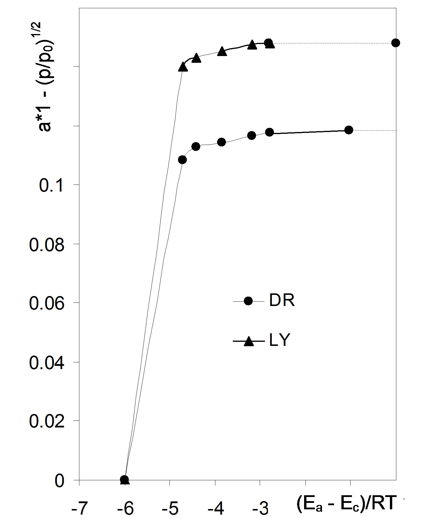
Figure 4. Dependence of monolayer adsorption on scaled adsorption energy for the studied root material. Dashed lines show monolayer capacity values. Abbreviations DR: average data from 36 isotherms for whole, cut, air dried and 105˚C dried roots, LY: average data from 18 isotherms for whole and cut lyophilized roots.
subranges equal to ΔE and estimation of f(Ei,av) for each subrange. Setting too narrow subranges makes no sense due to scattering of data points. We set ΔE equal to 1 scaled energy unit what is a rationale minimum and provides enough reproducibility of f(Ei) for the replicates of experimental data. The adsorption energy distribution functions for the studied roots are depicted in Figure 5.
Having calculated f(Ei) values, the average water vapor adsorption energy of the whole adsorbent, Eav, can be calculated as:
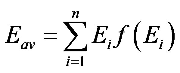 (7)
(7)
The average adsorption energy of the adsorbent can in principle be estimated also from the intercept of the linear plot of the Aranovich equation (Equation (1)), however frequently the estimated intercepts are close to zero, even negative, so the estimated adsorption energies are too high or unrealistic. The adsorption energy distribution function and average adsorption energy are sensitive to the calculation mode: less to selection of energy subranges and more to the choice of the highest adsorption energy value of the adsorbent, therefore for comparison of different materials and data taken in independent measurements, exactly that same calculation way should be applied.
3.2. Surface Fractal Dimension
General morphology of many natural surfaces is geomet-
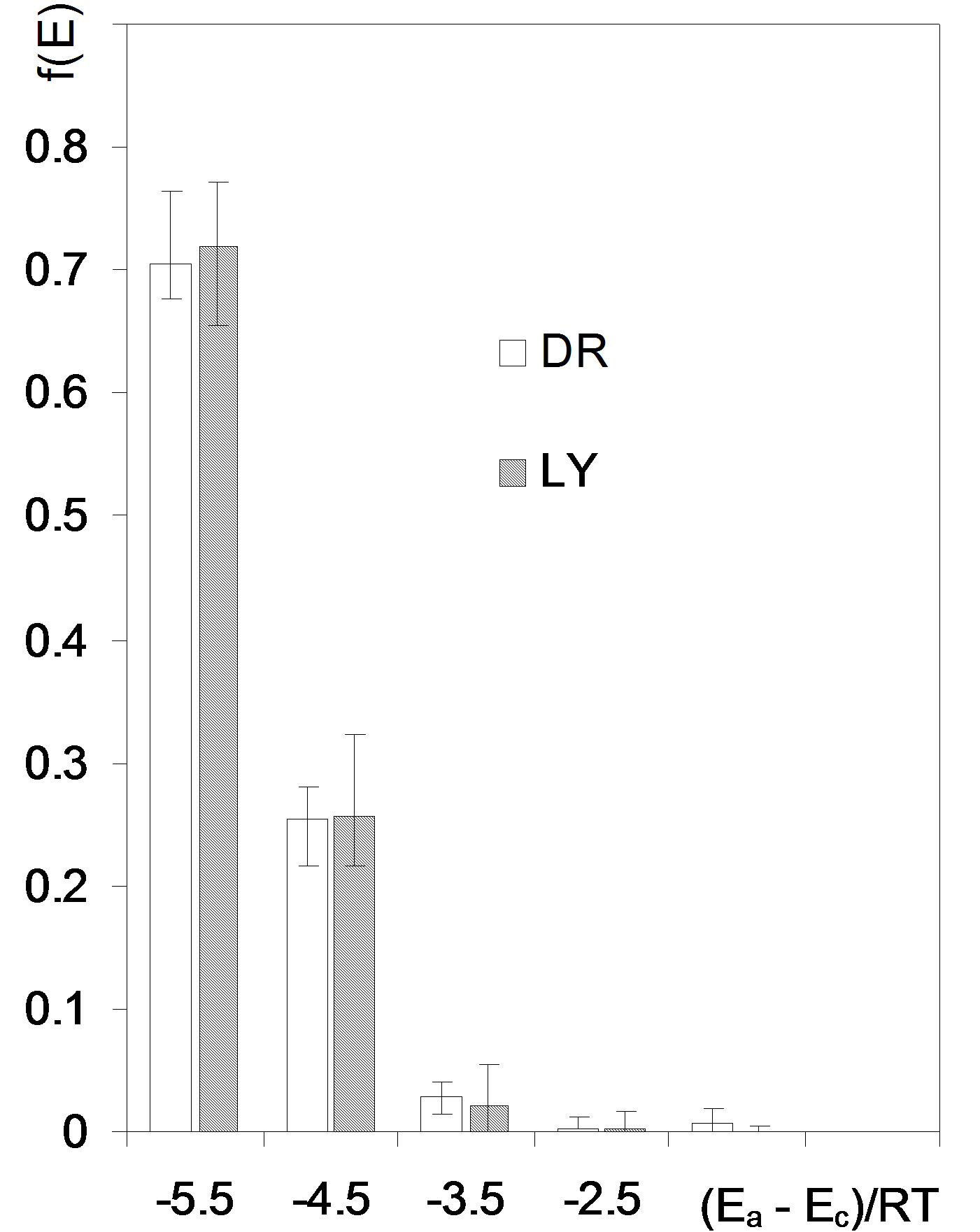
Figure 5. Adsorption energy distribution functions for the studied roots. Error bars show experimental deviations. Abbreviations DR: average data from 36 isotherms for whole, cut, air dried and 105˚C dried roots, LY: average data from 18 isotherms for whole and cut lyophilized roots.
rically similar at different levels of observation (magnification), and if so, the object displays fractal behavior [9]. As a rule, the fractal behavior of natural objects occurs in a limited range of scales, called upper and lower cutoffs [10]. A measure of the complexity of fractal structures is a fractal dimension, D, that is higher for more complex ones. As far as the fractal dimension is a single number parametrizing the complex structure in a broad size range, the theory of fractals has been widely used for describing structures of disordered media and processes occurring in them [11,12]. The surface fractal dimension, Ds, can be calculated from a single adsorption isotherm [13,14] by approximation of the experimentally measured adsorption versus relative pressure data by the equation:
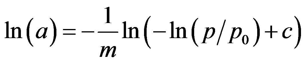 (8)
(8)
where c is a constant and m is a parameter. If the adsorbent displays fractal behavior, the plot of the above dependence displays a linear range, as this is shown in Figure 6 for the considered root materials.
Two regions of linearity of Equation (8) can be distinguished, however this equation should be applied to the experimental data measured within multilayer adsorption region, i.e. for relatively high relative pressures, wherein the effects of energetic surface heterogeneity play negligible role. Therefore the fractal behavior should be considered only for the region of high adsorption (left one in Figure 6). The parameter m calculated

Figure 6. Dependence of pore volume on pore radius. Note that zero pore volume locates at 1 nm pore radius. Abbreviations DR: average data from 36 isotherms for whole, cut, air dried and 105˚C dried roots, LY: average data from 18 isotherms for whole and cut lyophilized roots.
from the slope of the linear part of the above dependence is related to the surface fractal dimension. The magnitude of 1/m distinguishes two possible adsorption regimes [15]: for 1/m < 1/3, the adsorption occurs within van der Waals regime and the surface fractal dimension is:
 (9)
(9)
and for m > 1/3 the adsorption is governed by the capillary condensation mechanism and:
 (10)
(10)
Geometrical irregularities and roughness of the adsorbent surface have an essential influence on the value of the surface fractal dimension, which for solid surfaces may vary from 2 to 3. The lower limiting value of 2 corresponds to a perfectly smooth surface, whereas the upper limiting value of 3 relates to the maximum allowed surface complexity.
3.3. Nanopore Size and Size Distribution
Many natural bodies, including plant roots, are highly porous. The basic characteristic of porous bodies is provided by a pore size distribution function showing fractions of pores of different radii while the overall amount of the pores (total porosity) is estimated from the bulk density and the solid phase density of the material [16]. Total porosity value is of less importance for characteristic of porous materials because provides no information on pore dimensions and number. The same total porosity can result from small number of large pores and large number of small ones despite both above materials have quite different properties. More important pore characteristic is a pore size distribution function relating pore volumes and dimensions. The pore size distribution is determined using so called direct and indirect methods. Direct methods are based on an analyze of cross sections of porous bodies: nontransparent sections in reflected light and transparent ones in transmitted light microscopy. Image analyze of XRD and NMR scanning photographs is used, as well. Indirect methods determine pore size distributions basing on measurements of other physicochemical parameters related to pore sizes and volumes. The complicated pore shapes are usually approximated by selected geometrical models (slit-like, ink-bottle, conical, globular etc.), among which the most frequently used is a cylindrical pore model. Using water vapor desorption isotherms pores of nanometer-sizes can be characterized.
The water vapor condensed in a pore forms a lensshaped surface, called meniscus. The curvature of the meniscus depends somehow on the pore dimension. One relates these two values using any convenient pore model, which is selected either operationally or basing on a knowledge of the sample structure. As far as the model pore shape may not reflect the real pore shape, the pore dimensions calculated using models are called equivalent dimensions. Using desorption isotherms, the (cylindrical) pore radius r[m] can be related to the desorption pressure by the Kelvin equation [8,17]:
 (11)
(11)
where VW (m3·mole−1) is molar volume of water, sW (J·m−2) is water surface tension, and aW is a water-solid contact angle (assumed most frequently to be zero).
To find the amount of water vapor condensed in the adsorbent pores, the condensation range should be established. The lower limit of this range can be associated to a minimum pore radius able to condense water that can rationally be assumed as equal to 1 nanometer. Such pore is enough large to form a meniscus (the pore diameter of 2 nm equals to around 7 diameters of a water molecule). The radius of 1 nm corresponds to p/p0 ≈ 0.352 at T = 298 K, so the amount of the condensed vapor can be calculated as the adsorbate amount at a given p/p0 minus amount adsorbed at p/p0 ≈ 0.352. The amount (mass) a of condensed water may be expressed as the adsorbate volume v [m3] (v = a/d, where d [kg·m−3] is water density) that can be treated as the pore volume. Now one can plot the dependence of the pore volume to the pore radius that for the studied roots is shown in Figure 7.
The above dependence serves for estimation of distribution function of pore radii. The volume of the adsorbate filling the pores in a given range of radii is equal to the volume of these pores. Thus to find the volume v [m3·kg−1] of pores ranging between ri and ri + Δr a value of v(ri + Δr) minus v(ri) is calculated. Thus the fraction ni of i-th range pores is given by:
 (12)
(12)
where ri,av is the average pore radius equal to (r + r + Δr)/2 and vtot is the total volume of pores in the experimental window (from the assumed minimum r to the maximum r available from desorption data). In the present case the maximum value of r was set to 50 nm, because the maximum experimental p/p0 value of 0.98 corresponded to r ≈ 57 nm. Thus the distribution function of pore sizes is found by division of the whole experimental vapor condensation range on subranges equal to Δr and estimation of f(ri,av) for each subrange. Enough reproducibility of f(ri,av) for the replicates of experimental isotherms was reached setting the subranges of 10 nm (the first subrange was from 1 to 10 nm). The pore volume values for the boundary points of every subrange were estimated by linear interpolation of nearest desorption data. The pore size distribution functions of for the studied roots are depicted in Figure 8.
Having calculated f(ri,av) values, the average pore radius of the whole adsorbent, rav, can be calculated as:
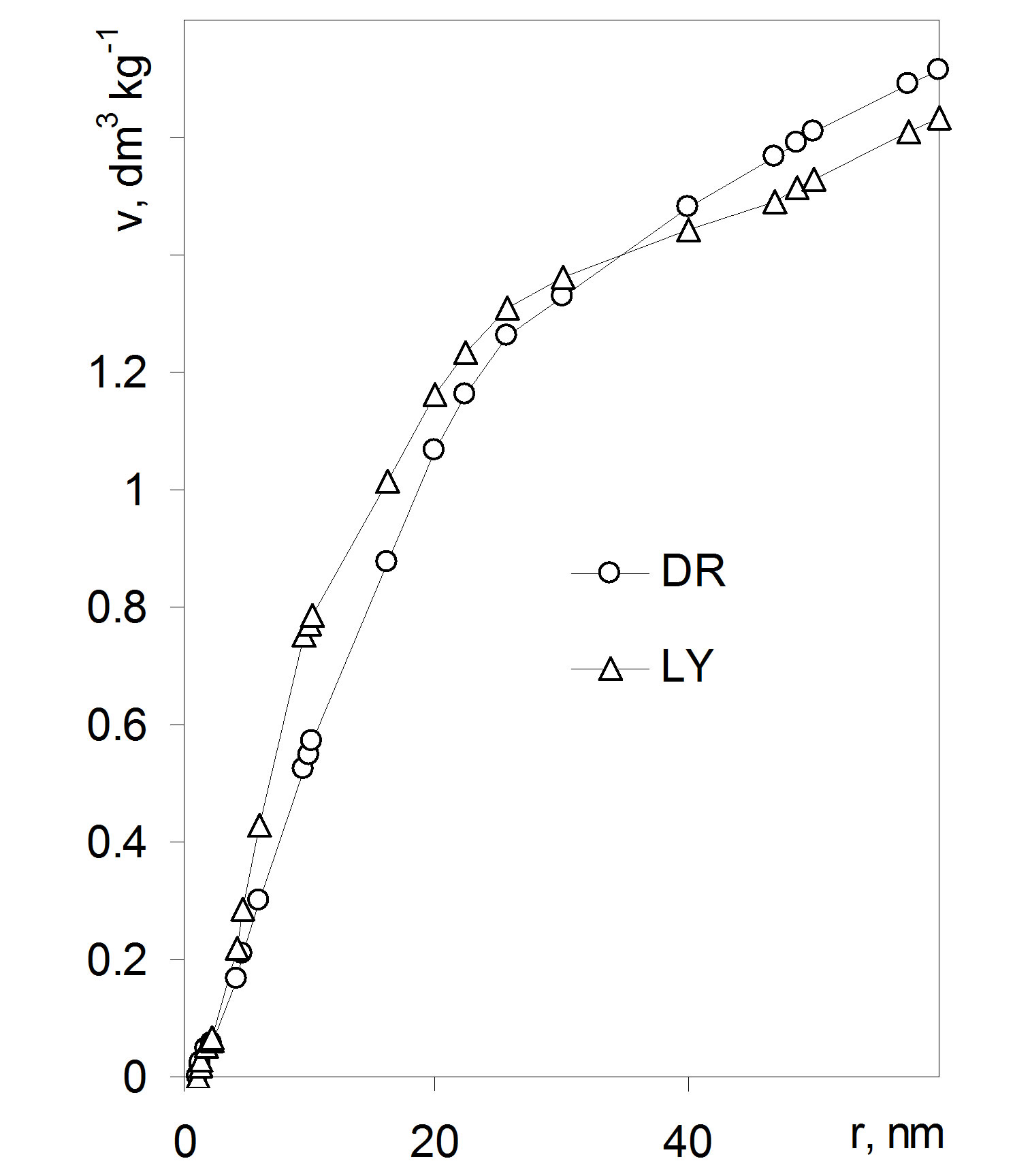
Figure 7. Nanopore size distribution functions for the studied roots. Error bars show experimental deviations. Abbreviations DR: average data from 36 isotherms for whole, cut, air dried and 105˚C dried roots, LY: average data from 18 isotherms for whole and cut lyophilized roots.
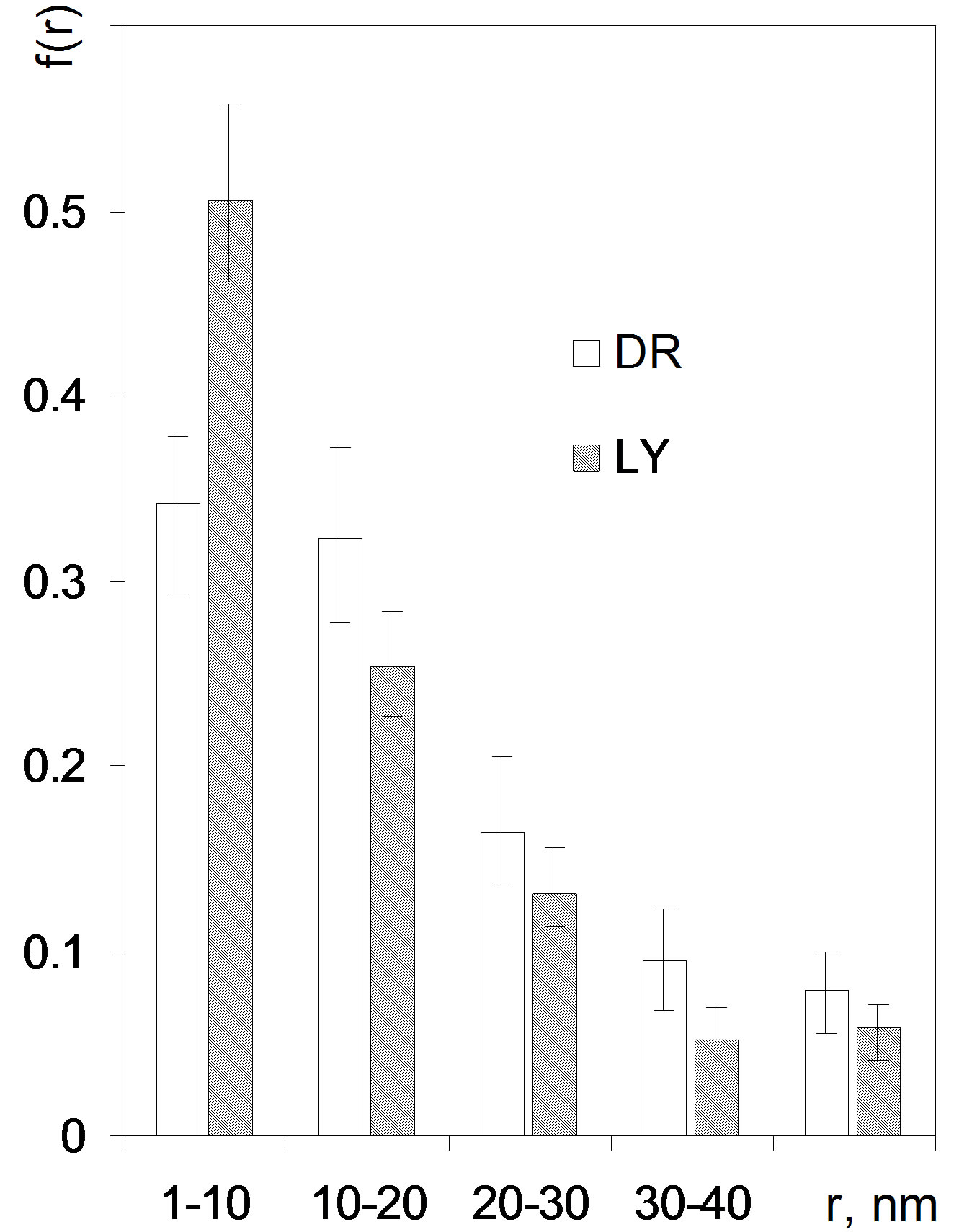
Figure 8. Fractal plot for the studied roots. Abbreviations DR: average data from 36 isotherms for whole, cut, air dried and 105˚C dried roots, LY: average data from 18 isotherms for whole and cut lyophilized roots.
 (13)
(13)
Very likely the “real” pores are larger than these calculated from Kelvin equation because before the condensation of water vapor, the pore walls are covered with a monolayer of adsorbed water. The thickness of this layer can be added to the equivalent pore radius to obtain more realistic value. The pore size distribution function and the value of average pore radius are sensitive to the calculation mode, especially to the choice of the largest pore radius, therefore for comparison of different materials and data taken in independent measurements, exactly that same calculation way should be applied.
Frequently in the literature the pore size fractions are related to log(r) and not to r values. In this case instead of average pore radius in Equation (13), the average log(rav) value is calculated. The average radius taken as 10^(log(rav)) gives lower values than rav because of lowering the input of large radii. The latter approach is more sound if pore size range covers a few orders of magnitude.
4. Results and Discussion
Values of surface characteristics of the considered roots are presented in Table 1. These data were calculated from 9 replicates of adsorption/desorption isotherms.
Water molecules are adsorbed stronger by the roots than by soils: adsorption energies of roots (over −5) are markedly higher than these for soils (from −1 to −3.5). As far as water adsorption energy reflects the overall
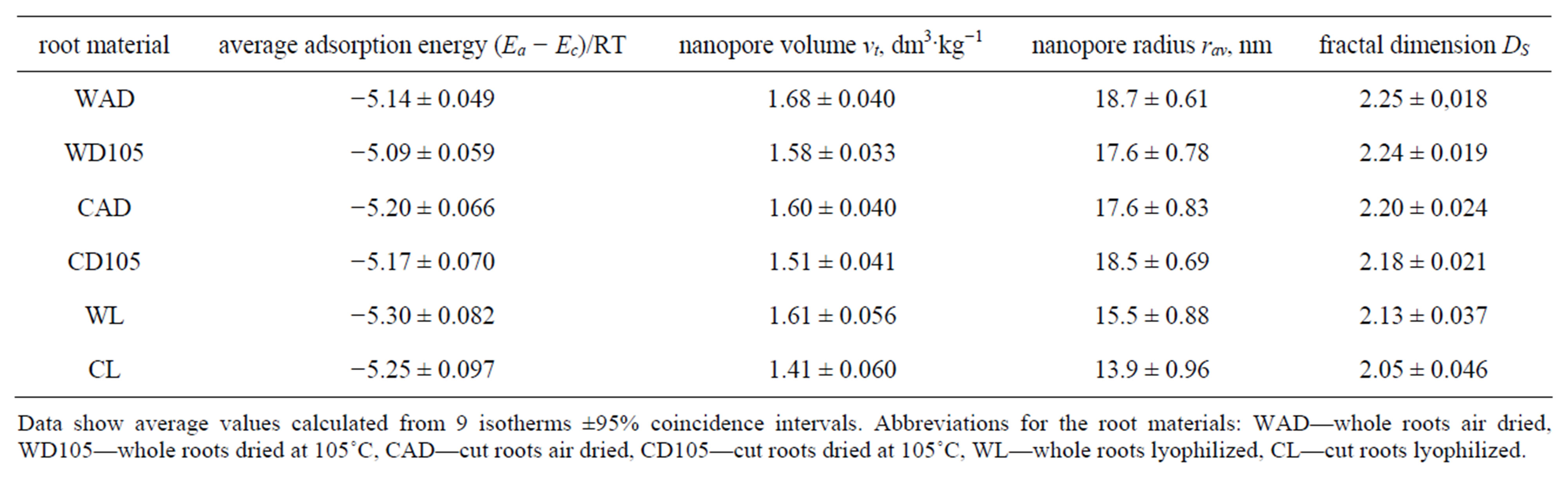
Table 1. Surface parameters of the studied roots.
Data show average values calculated from 9 isotherms ±95% coincidence intervals. Abbreviations for the root materials: WAD—whole roots air dried, WD105—whole roots dried at 105˚C, CAD—cut roots air dried, CD105—cut roots dried at 105˚C, WL—whole roots lyophilized, CL—cut roots lyophilized.
forces of water molecules binding to a surface, plants of higher adsorption energy of roots should better survive in low moisture environments and be more resistant to draught than plants of lower adsorption energy. To check this hypothesis we started to investigate energetic properties of roots of different varieties of barley of various tolerance to draught.
Plant roots are highly porous structures: the total volume of pores in 1 - 50 nm radii range exceeds 1.5 dm3 per kilogram of the roots. Including larger radii this can be markedly higher. Assuming the density of the solid phase of the root material as equal to around 1.5 kg·dm−3, one can state that the pore volume comprises at least half of the bulk material volume. Despite the average pore radius is high (around 17 nanometers) most of the pores are much smaller, as this is seen from pore size distributions. At present this is difficult to attribute the pores of a given radius to particular structural features of the roots anatomical components. Possibly simultaneous electronmicroscopic studies could give a better insight into the above problem, however, some comparisons may be drawn. The cell walls microfibrils are between 3 - 30 nm in diameter [18] so the pores formed within the microfibrils net can have radii of a few nanometers. The larger pores may constitute intercellular spaces. The pores of about 2 nm radius are reported to occur in the (radish and sycamore) apoplast [18]. Possibly similar pores might have been detected also from desorption isotherms. Such pores are important for ions and molecules transport processes in plants [18]. Anyway, the question whether plant root pores measured from water desorption are that same as measured by other methods e.g. osmotic permeability [19] or microscopy [20] remains opened.
Low values of the surface fractal dimensions indicate that root surfaces are rather smooth and not very complicated. Somewhat higher surface areas and adsorption energies together with lower pore sizes and fractal dimensions of lyophilized roots indicate that the history of pretreatment has some influence on the material structure. As the above effects are not high, air drying can be proposed as most convenient choice for preparation of root material for studying adsorption/desorption isotherms.
5. Conclusion
Water vapor adsorption/desorption isotherm is an easy tool to characterize physicochemical parameters of plant roots surface and of root nanopore system. These parameters may have some practical and theoretical importance for characterizing root surface properties, their changes in stress conditions, as well as to study and model plant processes, however much further work is needed to check these hypotheses.
6. Acknowledgements
This work was supported by the European Regional Development Fund through the Innovative Economy Program for Poland 2007-2013, project WND-POIG.01.03. 01-00-101/08 POLAPGEN-BD, Biotechnological tools for breeding cereals with increased resistance to drought”. The project is realized by POLAPGEN Consortium coordinated by Institute of Plant Genetics, Polish Academy of Sciences in Poznan. Further information about the project can be found at www.polapgen.pl.
REFERENCES
- G. Jozefaciuk and M. Lukowska, “New Method for Measurement of Plant Roots Specific Surface,” American Journal of Plant Sciences, Vol. 4, No. 5, 2013, pp. 1088- 1094. doi:10.4236/ajps.2013.45135
- G. L. Aranovich, “The Theory of Polymolecular Adsorption,” Langmuir, Vol. 8, No. 2, 1992, pp. 736-739. doi:10.1021/la00038a071
- S. Brunauer, P. H. Emmet and E. Teller, “Adsorption of Gases in Multimolecular Layers,” Journal of American Chemical Society, Vol. 60, No. 2, 1938, pp. 309-314. doi:10.1021/ja01269a023
- M. Jaroniec and P. Brauer, “Recent Progress in Determination of Energetic Heterogeneity of Solids from Adsorption Data,” Surface Science Reports, Vol. 6, No. 2, 1986, pp. 65-117. doi:10.1016/0167-5729(86)90004-X
- M. Jaroniec, W. Rudzinski, S. Sokolowski and R. Smarzewski, “Determination of Energy Distribution Function from Observed Adsorption Isotherms,” Journal of Colloid and Polymer Science, Vol. 253, No. 2, 1976, pp. 164-166. doi:10.1007/BF01775683
- P. Kowalczyk, H. Tanaka, H. Kanoh and K. Kaneko, “Adsorption Energy Distribution Function from the Aranovich-Donohue Lattice Density Functional Theory,” Langmuir, Vol. 20, No. 6, 2004, pp. 2324-2332. doi:10.1021/la035748k
- S. J. Gregg and K. S. W. Sing, “Adsorption, Surface Area and Porosity,” Academic Press, London, New York, 1967.
- J. Oscik, “Adsorption,” Ellis Horwood, Chichester, 1982.
- B. B. Mandelbrot “The Fractal Geometry of Nature,” Freeman, San Francisco, 1983.
- Y. A. Pachepsky, T. A. Polubesova, M. Hajnos, Z. Sokolowska and G. Jozefaciuk, “Fractal Parameters of Pore Surface Area as Influenced by Simulated Soil Degradation,” Soil Science Society of America Journal, Vol. 59, No. 1, 1995, pp. 68-75. doi:10.2136/sssaj1995.03615995005900010010x
- Y. A. Pachepsky, J. W. Crawfordf and W. J. Rawls, “Fractals in Soil Science,” Elsevier, Amsterdam, 2000.
- P. Pfeifer and M. Obert, “Fractals Basic Concepts and Terminology,” In: D. Avnir, Ed., The Fractal Approach to Heterogeneous Chemistry, J Willey and Sons, Hoboken, 1989, pp. 11-43.
- M. Jaroniec, “Evaluation of the Fractal Dimension from a Single Adsorption Isotherm,” Langmuir, Vol. 11, No. 6, 1995, pp. 2316-2317. doi:10.1021/la00006a076
- A. V. Neimark, “A New Approach to Determination of the Surface Fractal Dimension of Porous Solids,” Physica Acta, Vol. 191, No. 1-4, 1992, pp. 258-262. doi:10.1016/0378-4371(92)90536-Y
- A. B. Jarzebski, J. Lorenc and L. Pajak, “Surface Fractal Characteristics of Silica Aerogels,” Langmuir, Vol. 13, No. 5, 1997, pp. 1031-1035. doi:10.1021/la960011z
- R. Rouquerol, D. Avnir, C. W. Fairbridge, D. H. Everett, J. H. Haynes, N. Pernicone, J. D. F. Ramsay, K. S. W. Sing and K. K. Unger, “Recommendations for the Characterization of Porous Solids,” Pure and Applied Chemistry, Vol. 66, No. 8, 1994, pp. 1739-1758. doi:10.1351/pac199466081739
- K. S. W. Sing, “Reporting Physisorption Data for Gas/ Solid Systems with the Special Reference to the Determination of Surface Area and Porosity,” Pure and Applied Chemistry, Vol. 54, No. 11, 1982, pp. 2201-2218.
- D. T. Clarkson, “Root Structure and Sites of Ion Uptake,” In: Y. Weisel, A. Eshel and U. Kafkafi, Eds., Plant Roots The Hidden Half, Marcel Dekker, New York, 1991, pp. 351-373.
- N. Carpita, D. Sabulase, D. Montezinos and D. P. Delmer, “Determination of the Pore Size of Cell Walls of Living Plant Cells,” Science, Vol. 205, No. 4411, 1979, pp. 144- 147. doi:10.1126/science.205.4411.1144
- A. W. Robards, “Electron Microscopy and Plant Ultra Structure,” McGraw-Hill, New York, 1970.
NOTES
*Corresponding author.