Computational Water, Energy, and Environmental Engineering
Vol.07 No.01(2018), Article ID:81198,24 pages
10.4236/cweee.2018.71002
The Influence of Rain Gauge Network Density on the Performance of a Hydrological Model
George Andiego1, Muhammad Waseem2, Muhammad Usman3, Nithish Mani4
1Water Resources and Environmental Services Department, Nairobi, Kenya
2Faculty of Agriculture and Environmental Sciences, Universität Rostock, Rostock, Germany
3Institute of Water Resources and Water Supply, TUHH Hamburg, Am Schwarzenberg-Campus 3 (E), Hamburg, Germany
4Sahasrara Earth Services & Resources Ltd., Hanover, Germany

Copyright © 2018 by authors and Scientific Research Publishing Inc.
This work is licensed under the Creative Commons Attribution International License (CC BY 4.0).
http://creativecommons.org/licenses/by/4.0/


Received: November 16, 2017; Accepted: December 17, 2017; Published: December 20, 2017
ABSTRACT
Rain gauge data suffers from spatial errors because of precipitation variability within short distances and due to sparse or irregular network. Use of interpolation is often unreliable to evaluate due to the aforementioned irregular sparse networks. This study is carried out in the Nette River catchment of Lower Saxony to alleviate the problem of using gauge data to measure the performance of interpolation. Radar precipitation data was extracted in the positions of 53 rain gauge stations, which are distributed throughout the range of the weather surveillance radar (WSR). Since radar data traditionally suffers from temporal errors, it was corrected using the Mean Field Bias (MFB) method by utilizing the rain gauge data and then further used as the reference precipitation in the study. The performances of Inverse Distance Weighting (IDW) and Ordinary Kriging (OK) interpolation methods by means of cross validation were assessed. Evaluation of the effect of the gauge densities on HBV-IWW hydrological model was achieved by comparing the simulated discharges for the two interpolation methods and corresponding densities against the simulated discharge of the reference precipitation data. Interpolation performance in winter was much better than summer for both interpolation methods. Furthermore, Ordinary Kriging performed marginally better than Inverse Distance Weighting in both seasons. In case of areal precipitation, progressive improvement in performance with increase in gauge density for both interpolation methods was observed, but Inverse Distance Weighting was found more consistent up to higher densities. Comparison showed that Ordinary Kriging outperformed Inverse Distance Weighting only up to 70% density, beyond which the performance is equal. The hydrological modelling results are similar to that of areal precipitation except that for both methods, there was no improvement in performance beyond the 50% gauge density.
Keywords:
Gauge Density, Inverse Distance Weighting, Nette River, Ordinary Kriging

1. Introduction
Hydrological modelling to simulate historical discharges and to forecast future runoff is extensively used as a tool to understand catchment processes and to optimize water allocation and management. The gauge network is a key driver in hydrologic modelling to characterize discharge [1] . A real time rainfall estimation helps to predict groundwater recharge estimations under different hydrological conditions and plays even a vital role in agriculture water management (e.g. [2] [3] ). Rain gauges provide rainfall measurements at individual points but different uncertainties are associated with the use of gauge data to estimate rainfall with appropriate temporal and spatial scale variation at basin scale [4] . Even if rain gauges are equipped with real-time rainfall information at very fine temporal resolution under the help of automatic rainfall recording equipment, it is still a challenge to characterize the spatial variation of rainfall without a network of well-defined rain gauges in the catchment [5] . Accuracy of precipitation data input has a direct bearing on the performance of models. In many countries, the choice of the location of rain gauges is not planned nationally but rather is an ad-hoc localized process. This leads to irregular and inefficient allocation of gauges. To provide information in ungauged locations, physically- or statistically-based hydrological models are popular estimation tools [6] [7] . Due to the sparse or irregular location of the station, inherent error when carried forward to the hydrological process may lead to inaccurate hydrological modelling results. To anticipate spatial inaccuracies of gauge data, it was thought that with the introduction of precipitation measuring radar, continuous spatial information of precipitation could lead to more accurate measurements. Drop size and type of precipitation plays a major role as radar measures the precipitation on the basis of rainfall reflection rate intensities. Although radar provides precipitation information at longer ranges, higher temporal resolution and continuous spatial information also suffers measurement errors among which include clutter, bright band effect (a dark region in range height indication (RHI) scans due to melting of precipitation as it descends) and volume errors [8] .
Methods have been developed in several studies which either merge or interpolate data from the two measurement methods or correct the data using information from either measurement method. Merging or interpolation methods can either be univariate or multivariate. The common univariate methods are Nearest Neighbour, Thiessen Polygon and Inverse Distance methods, Ordinary Kriging (OK) and Indicator Kriging (IK) while the multivariate methods are Kriging with external Drift (KED) [9] . A review by Goudenhoofdt and Delobbe [10] discussed other methods such as Mean Field Bias Correction, Range dependant adjustment, Brandes Spatial Adjustment, Static local bias correction and range dependent adjustment (SRD), Ordinary Kriging, Conditional Merging and Kriging with external drift. To acquire spatially continuous precipitation information where only point data is available requires interpolation of the point data using the aforementioned methods. The accuracy of interpolation is usually determined using the cross validation method. However, if the distribution of the gauge stations is irregular or if they are too few, the results of the cross validation method become irrelevant because of non-representativeness [11] . In this situation, the determination of the interpolation accuracy can be evaluated by using the interpolated data as an input in a hydrological model. A study by Amin Daghighi [12] tested two machine learning techniques by using Stepwise Multiple Regression (SMR) and Genetic Programming (GP), to forecast monthly harmful algal blooms (HAB) indicators in Western Lake Erie from July to October. The SMR models showed a correlation coefficient increase from 0.71 to 0.78 when extending the training period. The GP models followed a similar trend increasing the overall correlation coefficient from 0.82 to 0.96. A study by Gascon et al. [13] used the data produced by a very dense rainfall network covering the Ouémé catchment in Benin and studied the impact of varying the spatial and temporal resolution of input rain fields on the output produced by DHSVM (Distributed Hydrology Soils and Vegetation Model), thus representing the resolution induced errors associated with using satellite rainfall input for physically based models. Result of this sensitivity analysis showed that the model output is more sensitive to the temporal resolution than to the spatial resolution, at least for this region and for the range of resolutions tested. A study by Buytaert et al. [14] in the Ecudarian highlands showed OK performed better than Thiessen Polygon. Goovaert [15] compared multivariate Kriging methods with additional elevation information against univariate IDW, Thiessen polygon and OK methods with the two deterministic methods performing worst. However other studies such as Otieno et al. [16] in a British catchment showed that OK and IDW performed similarly well. Study compared the influence of three different gauge densities on performance of a geostatistical and deterministic interpolation methods and found progressive improvement in performance with every increase in gauge density. Dirks et al. [17] compared Kriging method with IDW, Thiessen and Areal mean method in a catchment with dense gauge network and the results showed IDW performed best. The influence of precipitation interpolation methods on hydrological modelling results show mixed results. A study using the Hydrostrahler model in a West African catchment by Ruelland et al. [18] showed that the IDW method performed much better than OK and Thiessen methods. Haberlandt and Kite [19] using the SLURP model compared geostatistical and deterministic methods found the former performing better. A similar study by Villarini et al. [20] evaluated the effect of both temporal resolution and gauge density on the performance of remotely sensed precipitation products and the results showed progressive improvement with increasing density. Similar studies with similar results were carried out by Berndt et al. [21] which compared among other things the influence of temporal resolution and gauge density on variety of interpolation methods. Duncan et al. [22] , using only Thiessen interpolation method, evaluated the effect of gauge density on a hydrological model with results indicating performance improves with increase in density by a power law. The results were not so definitive in a study by Krajewski et al. [23] where two models and temporal resolution of precipitation input and the gauge density were compared. Results showed that the higher the gauge counts the better the simulation accuracy and improvement was not dramatic between low and high densities. From the foregoing, it is apparent that studies to determine the best methods of merging radar and rain gauge precipitation data, the accuracy of rainfall interpolation methods, the influence of gauge density on hydrological models have been carried out. However, studies to evaluate the influence of rain gauge density and interpolation methods on the performance of hydrological models are missing.
This study is based in the Nette River catchment in the Lower Saxony state of Germany. It is a small catchment of approximately 300 km2 within the range of the Hannover weather radar which covers a radius of 128 km. The precipitation data of the period between 2006 and 2010 from the radar station was interpolated after being extracted at the locations of the rain gauge stations, totalling 53, within its coverage. To reduce the temporal inaccuracies inherent in radar data before the extraction of the radar data, it was corrected using the Mean Field Bias (MFB) method and aggregated from five minute to hourly precipitation. The extracted and corrected radar data was then used as the reference precipitation data against which the performance of the interpolated data was compared. The performance of two interpolation methods, Ordinary Kriging (OK) and Inverse Distance Weighting (IDW), were compared by means of Cross Validation method. The problem of non-representativeness is avoided because the interpolated data is compared against the spatially continuous radar. As the use of radar for precipitation measurement is influenced by the drop size, seasonal variation of precipitation type in summer and winter affects accuracy of measurement. Therefore, the effect of seasons on interpolation was examined. The rain gauge densities chosen for this study were 25%, 50%, 70%, 80%, and 100%. For each density, the equivalent number of gauges was randomly picked ten times so that each interpolation method had 41 data series. This was then used to calculate areal precipitation for the study area and eventually hydrological modelling using the HBV-IWW model.
The HBV-IWW hydrological model is a conceptual, semi-distributed hydrological model. It is partitioned into snow, soil and response routine. The inputs required in the model include surface temperature, areal precipitation, potential evapotranspiration, actual evapotranspiration and soil moisture content. Required parameter includes soil field capacity, soil runoff threshold, wet snow melt factor (wsmf), threshold temperature, and shape response parameter. For the river routing routine, the Muskingum method is used. Usually evaluating model performance involves comparing actual observed discharge against the simulated discharge. This process involves calibration and validation of the parameters to best describe modelled catchment conditions. In contrast, this study used previously determined optimum parameters and no calibration or validation carried out. This is because the comparison was not against actual measured discharge but against the discharge from the reference precipitation data. This means that for every sub-catchment, the only input or parameter that changed is the precipitation data. The simulated discharge from modelling using precipitation data from the two interpolation methods and the different gauge densities were therefore compared with those from the reference precipitation data to evaluate the main objective of the study.
2. Materials and Methods
2.1. Location, Climate, Hydrology and Topography
The basin area under study is the Nette River catchment. It is located in the Northern part of Germany in the state of Lower Saxony as illustrated in Figure 1 (left). It is part of the larger Wesser River system and covers an area of 49,000 km2. The main tributary of the Wesser River system is the Aller River, of which the Leine River is a major tributary.
The Aller/Leine River basin is located in the South-Eastern part of Niedersachsen with an area of over 15,803 km2. The elevations in the basin range between 5 masl near the outlet to the North Sea to 1140 masl at the headwaters in the Harz Mountains. Land use at the headwaters is mainly forestation. The annual precipitation is high and is characterised by frost in winter the season. Agriculture uses approximately 58.2% of the land while forests cover another 32.5% [24] . Nette River basin lies between the Northing 5,743,100 and 5,773,700 and Easting 3,571,200 and 3,586,900 (Deutsces_Hauptdreiecksnetz_Transverse_Mercator coordinate system). The basin has an area of approximately 300 km2 measured at the Derneburg river gauging station (No. 4886156). The mean basin elevation is 206 masl. The highest elevation of the basin is approximately 621 masl and 92 masl at the lowest location shown in Figure 1 (right). The Nette basin climate characteristics are of a typical temperate oceanic with pronounced winter and summer seasons. Mean annual precipitation and mean monthly temperature is 872 mm and 9.29 degrees Celsius respectively [25] . The climate graph of the nearby Hannover City in Figure 2 shows increased precipitation in the summer months, high frost and relative humidity in winter and near equal average wind speed throughout the year.
2.2. Description of the Data
2.2.1. Precipitation
There are 53 rain gauge stations and one radar station data used in the study. The radar coverage range is 128 km, and all the gauge stations are within the

Figure 1. Location of the Nette River basin (left) and Nette River basin topography (right).

Figure 2. Hannover city climate graph [26] .
circumference, as shown in Figure 3, with data for a period of five years (2006-2010). Both sets of data are of 5-minute temporal resolution, although this was later aggregated to hourly resolution during analysis. Only one rain gauge station is located within the study basin. The rain gauge information is only used to extract the radar precipitation data.
2.2.2. Correction of Radar Data
Radar precipitation data is prone to errors such as ground clutter, anomalous
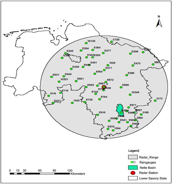
Figure 3. Rain gauge and radar location.
propagation, non-precipitation signals and bright band effects (due to melting of precipitation as it descends). During the same precipitation event, the drop size distribution within the storm can vary. This phenomenon introduces random multiplicative bias in the radar precipitation measurement. Satellite-based quantitative precipitation estimate (QPE) is associated with various uncertainties such as the errors in bias correction processes, observation and satellite retrieval [27] . The quality of satellite-based QPEs not only affects the precipitation distribution accuracy, but also effects the hydrologic outputs through interaction with the hydrologic processes in hydrologic models ( [28] [29] ). Because of the multiplicative errors inherent in radar data, it causes underestimations and overestimations. To correct this, two methods can be applied: merging it with gauge data sets or using the gauge data to correct it. To merge the two datasets, methods such as Co-Kriging, Kriging with External Drift [9] , Conditional Merging [21] have been used to transform the radar data according to gauge data, Box-Cox transformation, Q-Q transformation [30] . In this study, the Mean Field Bias Correction method advanced by Chumchean et al. [31] was used.
2.2.3. Mean Field Bias Correction (MBF)
Rain gauge precipitation data often suffers from spatial inaccuracies while radar data suffers from temporal errors. A study by Berndt et al. [21] compared the performance of gauge only data and merged gauge-radar precipitation data. The results showed that smoothed/merged data performed much better than the gauge only data. Before the merging of radar and rain gauge data, the radar data has to be adjusted using rain gauge data as the reference. Even before merging, preliminary treatment of the radar data includes correction for occultation, clutter, attenuation and range effects [32] . According to Chumchean et al. [31] , the improvement or correction of radar precipitation data can be summarized in the three steps: correction of range dependant errors, the correction of the reflectivity-rainfall/precipitation (Z-R) and finally Mean Field Bias Correction. The first two steps are usually carried out at the source of the radar data by the measuring agency.
MFB correction method is defined by the assumption that there is a systematic multiplicative difference between measured rain gauge data and radar data at a specific location. It therefore estimates this difference as shown in Equation (1) by summing up the gauge and radar readings and dividing to measure the underestimation or over-estimation coefficient:
(1)
where,
Gi―The rain gauge rainfall values (Daily);
Ri―The uncorrected radar rainfall raster values (Daily);
Ns―The number of gauge stations;
CMFB―The resulting co-efficient.
The values less than one show underestimations by the radar while values higher than one show overestimations. The calculation is carried out by summing up the daily precipitation values in both data sets in the location of rain gauge stations. The subsequent ratio from the calculation is then used to multiply and therefore correct the radar raster data which was in five-minute resolution for the applicable day as shown in Equation (2):
(2)
where,
Rcorrected―The corrected radar data (5 minute);
CMFB―The MFB correction coefficient (Daily);
Ri―The uncorrected radar data (5 minute).
The MFB (CMFB) coefficient calculation can result into unrealistically high and low values because of extreme errors. This necessitates restriction to a certain range hence the three scenarios which were tested in the project.
2.2.4. Mean Field Bias Options
The MFB correction does not correct all errors. Indeed, Chumchean et al. [31] , discusses some errors which are not rectifiable by MFB such as radar range errors, sampling errors and those due to electrical operation of the radar machines such as electrical calibration and quantification. Because of the uncorrected errors, the resulting MFB corrections coefficients can result in the errors being carried forward and this has the potential of lowering the accuracy of the corrected data. The MFB coefficient was used to correct the radar data which was then used as the reference precipitation data. This means that if the coefficient is unrealistic and therefore wrong, the error would be transferred to the corrected radar data (reference precipitation data) which would eventually affect the performance of the interpolation methods, mostly negatively. In order to alleviate this, the optimum MFB coefficient ranges have to be chosen by restricting the ratio within certain ranges. Therefore, three MFB co-efficient scenarios were created to test the significance of this effect by restricting the coefficients within a certain ranges. The three scenarios were:
Scenario 1: No restriction (0.0005 - 1000);
Scenario 2: Removal of outlier coefficients in Scenario 1 (0.5 - 8);
Scenario 3: Smallest range (0.5 - 3).
The test was done by randomly selecting and comparing three rain gauges and extracted radar stations for goodness of fit. After choosing Scenario 2, all the resulting MFB coefficients were restricted within the range (0.5 - 8) even if they were higher or lower than this. The coefficients were then applied to the radar data by multiplication in all the time steps. After the bias correction, the radar data was aggregated from five minute resolution to hourly resolution in order to match it with the other data which was used in the hydrological modelling process such as temperature and evaporation. The corrected and aggregated data was then designated the reference precipitation data and considered as the actual ground precipitation measurements.
2.2.5. Extraction of Radar Data
In order to evaluate the performance of the two interpolation methods under consideration in the study, the reference data was extracted into specific points before later interpolating the same data. The extraction process was done by using the rain gauges locations shown in Figure 3. For every location of 53 rain gauges, the precipitation data in the reference radar pixels were extracted, and it was now in point format just as the rain gauge data.
2.3. Interpolation Methods
The methods which have been used to interpolate precipitation in past studies can be broadly classified as univariate and multivariate. The common univariate methods are Nearest Neighbour, Thiessen Polygon and Inverse Distance methods, Ordinary Kriging (OK) and Indicator Kriging (IK) while the multivariate methods are Kriging with external Drift (KED) [9] . In this study, the extracted radar data was interpolated by using only the univariate methods of Inverse Distance Weighting (IDW) and Ordinary Kriging (OK), which can also be classified as deterministic and geostatistical methods respectively. The interpolation was carried out for the whole area covered by the stations. After interpolation, the performance of the two interpolation methods of IDW and OK was determined using cross validation. It is carried out by dropping the observed or reference data, re-estimating using the interpolation method chosen (OK or IDW) and comparing the estimated and the original data using the objective functions i.e. the Leave One Out method. This is done for all the gauge stations without replacement. The cross validation results for both seasons were compared vis-à-vis the interpolation methods. For each interpolation method, the reference data was compared with station densities of 25%, 50%, 70%, 80%, and 100% which means the number of gauges in comparison were 14, 27, 38, 43, and 53 respectively. The specific gauge stations in each density scenario were randomly selected, and each scenario had ten random selections in order to avoid any bias. This means that each interpolation method had 41 selections including the 100% scenario. Aerial precipitation was carried out only on the delineated catchment of Nette River. The precipitation was allocated on the ten sub-basins of the catchments. As part of the evaluation, aerial precipitation was calculated for IDW and OK interpolated precipitation. This was then evaluated with that of reference precipitation for goodness of fit.
2.4. HBV-IWW Model Setup
In order to set up the hydrological model and to evaluate both areal precipitation and hydrological model performance, the Nette River basin was delineated using the ArcMap 10 terrain processing function. The open source digital terrain models (DTM) i.e. SRTM90 were used as the elevation input. Once the whole basin was delineated, it was divided into ten sub-basins of roughly equal areas as shown in Figure 4. Table 1 shows the areas of all ten sub catchments in the Nette River basin.
Initial meteorological conditions differ for all the sub-catchments. This would have an effect on the output discharge from the model. This necessitated the preparation of an artificial training period. It was simply done by duplicating the year 2006 inputs so that the model starts to run from the artificial year of 2005. This resulted into steady state conditions for all the sub-basins when the year 2006 simulation started.
2.5. Performance Measurement
Traditional goodness of fit evaluation is used to measure the ability of a model to reproduce historical observed discharges, compare performance during calibration or to compare present performance against past performance [33] . In addition to the hydrological model performance assessment, efficiency criteria used are Nash and Sutcliffe (NSE), Root Mean Square Error (RMSE), Co-efficient of determination (R2) and Percent Bias (Pbias). Table 2 shows the efficiency criteria

Figure 4. Nette River basin sub-catchments.

Table 1. Nette basin sub-catchment areas.
used to measure each objective.
3. Results and Analysis
3.1. Mean Field Bias
The results in Figure 5 show that the restriction of MFB coefficients has negligible effect on the accuracy of the correction process. Scenario 1 (range 0.0001 - 1000) and Scenario 2 (range 0.005 - 8) perform similarly while Scenario 3 (range 0.5 - 3), which is the narrowest, was marginally worse. It can be concluded that although the effect is negligible, it is advisable to leave the range to be as wide as possible and not restrict it.
3.2. Interpolation and Cross Validation
Variograms
The first step in variogram analysis was to test for anisotropy by calculating experimental variograms for the extracted radar data and varying the azimuthal angles. The directional bands are defined by azimuth and dip angles considering the area geology. A tilt may also be incorporated to rotate the tolerance parameters about the calculation direction axis. The angles tested were 0 degrees, 45 degrees and 90 degrees. Figure 6 illustrates the results of two tests for anisotropy for a winter and summer period in the same year (2006).
Table 2. Performance objectives and efficiency criteria.

Figure 5. Performance of MFB scenarios.

Figure 6. Variogram plots of tests for anisotrop.
Precipitation data shows isotropy so that the spatial co-relation is only dependant on distance between the stations and not on the direction. After confirming isotropy, the 45 degree azimuth angle was chosen to calculate the experimental variograms for the whole time series (2006-2010). Different experimental variograms were then calculated for specific summer and winter seasons for the whole time series. The summer season ran from April to September of the same year while winter was from October to March of the following year. Theoretical variograms were then fitted out manually on the experimental variogram using the exponential model for the different seasons. An example of fitting a theoretical variogram to an experimental one for the first two seasons in 2006 of the time series is shown in Figure 7.
3.3. Cross Validation
To determine the accuracy of interpolating methods, the cross validation method was applied seasonally. A comparison was made on the performance between the winter and summer seasons. The performance of OK method is shown in Figure 8, while IDW method performance is shown in Figure 9.
The analysis shows a clear trend by season for both interpolation methods. The different objective functions give similar but different results. In case of RMSE, OK performance in winter season was better than summer seasons across the board. A similar performance is observed for IDW. PBIAS gives contrary results to the other three functions as it shows better performance in summer rather than winter for both OK and IDW methods. NSE winter season performance was better than summer for both interpolation methods. R2 performance was better in winter season than summer season throughout the study series for both OK and IDW. Figure 10 combines the performances of both interpolation methods into one seasonal box plot and compares summer (S1, S2, …etc.) and winter (W1, W2, …etc.) season performance. Naturally the results are similar to the previous analysis, and winter performance is better than those of summer season.

Figure 7. The fitting of a theoretical variogram on an experimental variogram.

Figure 8. Performance of OK method by cross validation.

Figure 9. Performance of IDW method by cross validation.

Figure 10. Seasonal performance of interpolation.
A box plot comparison of the performance of the two interpolation methods was done and resulted that, in the case of RMSE, OK method performs marginally better than IDW in both winter and summer season. PBIAS, the IDW method performed better than OK in winter and with a slight difference in summer. This contradicts the results of other objective functions. While in case of NSE, the OK method performed marginally better than IDW in winter but performed much better in summer. R2, the OK method performed marginally better than IDW in both winter and summer season. Figure 11 below shows the comparison of the interpolation methods by season.
3.4. Areal Precipitation Performance
Station density interpolation was carried out by taking different number of stations of the extracted interpolated radar data and the reference data and calculating the areal precipitation of the sub-basins of the delineated Nette River basin.
For the OK interpolation method, the following conclusions resulted, as illustrated in Figure 12, that in case of RMSE, there is a marked performance improvement from 25% to the other densities. Between 50% density and 80% density

Figure 11. Comparison of the interpolation methods by season.

Figure 12. Performance by gauge density of OK.

Figure 13. Performance by gauge density of IDW.
there is a marginal progressive improvement. However, the 100% density breaks the trend and shows significant increase. PBIAS performance results are similar to the previous measure except for the 100% density showing dramatically lower performance. NSE 25% density shows low performance followed by a significant and progressive increase for 50%, 70%, and 80%. The 100% density performs better than the middle three. R2 shows similar performance as RMSE and NSE objective functions.
In evaluating IDW as shown in Figure 13, RMSE shows graduated performance so that 25% has the worst performance which significantly improves for 50% and 60% and a further significant improvement for 80%, and 100%. PBIAS showed different performance with almost equal performance for 25%, 50%, and 70%. The 80% has the best performance, marginally better than the 100% density. NSE performance with 25% at the bottom, 50% and 70% with similar performance and 80%, and 100% performing at the same level. R2, performance is similar to NSE function. The conclusion to be drawn from the IDW analysis is that the higher the gauge density the higher the performance. However, it also indicates that there is marginal performance improvement between 50% & 70% density and 80% & 100% densities. An evaluation to determine the performance of the two interpolation methods was carried out vis-à-vis the station gauge density and as the results are represented in Figure 15.
Figure 14 showed a clear superior performance of the OK method over the

Figure 14. Comparison of areal precipitation performance of OK and IDW by density.
IDW over the gauge densities of 25%, 50% and 70%. However, there is equal performance at gauge densities of 80% and 100%. It can be therefore that for sparsely gauged catchments, OK method is the better interpolation method while for well-gauged basins either method can be used without loss of accuracy.
3.5. Hydrological Modelling Performance
Influence of both the gauge density and interpolation methods on the performance of the HBV-IWW hydrological model when compared to the runoff from the reference precipitation. The analysis for the OK method shows similarity with results of the areal precipitation as evidenced by Figure 15. All the objective functions are show similar results with the 25% density showing the worst performance and a marginal graduated improvement in performance of the other densities. Although the 100% density shows the best performance, it can be concluded that for hydrological modelling, there is no marked improvement in accuracy between 50% and 100% gauge density.
The results obtained for IDW interpolation method are almost similar to those of OK. The only difference is that whereas the OK method had marginal differences for the higher densities, the IDW show little difference between 50%, 70%, 80% and 100%. It can be concluded that higher densities more than 50% do not improve model performance. This is represented in Figure 16.
A direct comparison of the two interpolation methods shown in Figure 17, indicates that OK performs better than IDW for all the gauge densities and by all

Figure 15. Discharge performance of OK by density.

Figure 16. Discharge performance of IDW by density.

Figure 17. Comparison of model runoff performance of OK and IDW by density.
the objective functions. This differs from the areal precipitation results where for the higher densities, the performance of both interpolation methods the same by all the objective functions was.
4. Conclusions and Recommendations
In correcting the radar data using gauge data by means of the Mean Field Bias (MFB) Correction method, in theory, if the calculated coefficients are extremely high, would affect the accuracy of correction. However, results showed that there is no discernible effect on the accuracy of correction. In fact, the opposite is true; that if the coefficients are restricted to narrower smaller values, the correction is much worse. On the seasonal variation of performance of precipitation interpolation method: 1) The performance in winter was better than in summer for both OK and IDW. This can attribute to the precipitation type difference as snow particles leads to better radar measurements in winter than summer; 2) OK performed better than IDW method in both summer and winter.
On the performance with different rain gauge density scenarios: 1) For OK, the performance improved significantly from gauge density of 25% to 50% and minimal improvement for higher densities; 2) For IDW, the performance improved significantly from gauge density of 25% to 80% and marginally thereafter; 3) When direct performance comparison was made between OK and IDW, the OK performed better than IDW for gauge densities between 25% - 70%. It can be concluded therefore that OK is the recommended interpolation technique for lower densities and the simpler IDW for higher densities.
The results for hydrological modelling show similar results as interpolation performance. The optimum gauge density for modelling is 50% as higher densities do not improve performances. The OK method is the best interpolation method for good model simulation compared to IDW. Since this study was carried by comparing the performance of interpolation methods against a reference precipitation data, future studies can be designed to test for interpolation performances against actual discharge measurement.
Acknowledgements
We would like to thank especially Prof. Dr. Haberlandt, Mr Berndt and Mr Rabieifor their guidance and help [Leibniz Universität Hannover]. We also would like to thank everybody who has helped and guided us towards improvement of this study.
Conflicts of Interest
The authors declare no conflict of interest.
Cite this paper
Andiego, G., Waseem, M., Usman, M. and Mani, N. (2018) The Influence of Rain Gauge Network Density on the Performance of a Hydrological Model. Computational Water, Energy, and Environmental Engineering, 7, 27-50. https://doi.org/10.4236/cweee.2018.71002
References
- 1. Shope, C.L. and Maharjan, G.R. (2015) Modeling Spatiotemporal Precipitation: Effects of Density, Interpolation, and Land Use Distribution. Advances in Meteorology, 2015, Article ID: 174196. https://doi.org/10.1155/2015/174196
- 2. Merayyan, S. and Safi, S. (2014) Feasibility of Groundwater Banking under Various Hydrologic Conditions in California, USA. Computational Water, Energy, and Environmental Engineering, 3, 79. https://doi.org/10.4236/cweee.2014.33009
- 3. Daghighi, A., Nahvi, A. and Kim, U. (2017) Optimal Cultivation Pattern to Increase Revenue and Reduce Water Use: Application of Linear Programming to Arjan Plain in Fars Province. Agriculture, 7, 73. https://doi.org/10.3390/agriculture7090073
- 4. Xu, H. (2015) Impact of Density and Location of Rain Gauges on Performances of Hydrological Models.
- 5. Xu, H., Xu, C.Y., Saelthun, N.R., Xu, Y., Zhou, B. and Chen, H. (2015) Entropy Theory Based Multi-Criteria Resampling of Rain Gauge Networks for Hydrological Modelling—A Case Study of Humid Area in Southern China. Journal of Hydrology, 525, 138-151. https://doi.org/10.1016/j.jhydrol.2015.03.034
- 6. Booker, D.J. and Woods, R.A. (2014) Comparing and Combining Physically-Based and Empirically-Based Approaches for Estimating the Hydrology of Ungauged Catchments. Journal of Hydrology 508, 227-239. https://doi.org/10.1016/j.jhydrol.2013.11.007
- 7. Archfield, S.A., Clark, M., Arheimer, B., Hay, L.E., Farmer, W.H., McMillan, H., Seibert, J., Kiang, J.E., Wagener, T., Bock, A., Hakala, K., Andréassian, V., Attinger, S., Viglione, A., Knight, R.R. and Over, T.M. (2015) Accelerating Advances in Continental Domain Hydrologic Modeling. Water Resources Research 51, 10078-10091. https://doi.org/10.1002/2015WR017498
- 8. Chandrasekar, V. and Cifelli, R. (2012) Concepts and Principles of Rainfall Estimation from Radar: Multi Sensor Environment and Data Fusion. Indian Journal of Radio & Space Physics, 41, 389-402.
- 9. Haberlandt, U. (2007) Geostatistical Interpolation of Hourly Precipitation from Rain Gauges and Radar for a Large-Scale Extreme Rainfall Event. Journal of Hydrology, 332, 144-157. https://doi.org/10.1016/j.jhydrol.2006.06.028
- 10. Goudenhoofdt, E. and Delobbe, L. (2009) Evaluation of Radar-Gauge Merging Methods for Quantitative Precipitation Estimates. Hydrology and Earth System Sciences, 13, 195-203. https://doi.org/10.5194/hess-13-195-2009
- 11. Wagner, P.D., Fiener, P., Wilken, F., Kumar, S. and Schneider, K. (2012) Comparison and Evaluation of Spatial Interpolation Schemes for Daily Rainfall in Data Scarce Regions. Journal of Hydrology, 464, 388-400. https://doi.org/10.1016/j.jhydrol.2012.07.026
- 12. Daghighi, A. (2017) Harmful Algae Bloom Prediction Model for Western Lake Erie using Stepwise Multiple Regression and Genetic Programming.
- 13. Gascon, T., Vischel, T., Lebel, T., Quantin, G., Pellarin, T., Quatela, V., Galle, S., et al. (2015) Influence of Rainfall Space-Time Variability over the Ouémé Basin in Benin. Proceedings of the International Association of Hydrological Sciences, 368, 102-107. https://doi.org/10.5194/piahs-368-102-2015
- 14. Buytaert, W., Celleri, R., Willems, P., De Bievre, B. and Wyseure, G. (2006) Spatial and Temporal Rainfall Variability in Mountainous Areas: A Case Study from the South Ecuadorian Andes. Journal of Hydrology, 329, 413-421. https://doi.org/10.1016/j.jhydrol.2006.02.031
- 15. Goovaerts, P. (2000) Geostatistical Approaches for Incorporating Elevation into the Spatial Interpolation of Rainfall. Journal of Hydrology, 228, 113-129. https://doi.org/10.1016/S0022-1694(00)00144-X
- 16. Otieno, H., Yang, J., Liu, W. and Han, D. (2014) Influence of Rain Gauge Density on Interpolation Method Selection. Journal of Hydrologic Engineering, 19, Article ID: 04014024. https://doi.org/10.1061/(ASCE)HE.1943-5584.0000964
- 17. Dirks, K.N., Hay, J.E., Stow, C.D. and Harris, D. (1998) High-Resolution Studies of Rainfall on Norfolk Island: Part II: Interpolation of Rainfall Data. Journal of Hydrology, 208, 187-193. https://doi.org/10.1016/S0022-1694(98)00155-3
- 18. Ruelland, D., Ardoin-Bardin, S., Billen, G. and Servat, E. (2008) Sensitivity of a Lumped and Semidistributed Hydrological Model to Several Methods of Rainfall Interpolation on a Large Basin in West Africa. Journal of Hydrology, 361, 96-117. https://doi.org/10.1016/j.jhydrol.2008.07.049
- 19. Haberlandt, U. and Kite, G.W. (1998) Estimation of Daily Space-Time Precipitation Series for Macroscale Hydrological Modelling. Hydrological Processes, 12, 1419-1432. https://doi.org/10.1002/(SICI)1099-1085(199807)12:9<1419::AID-HYP645>3.0.CO;2-A
- 20. Villarini, G., Mandapaka, P.V., Krajewski, W.F. and Moore, R.J. (2008) Rainfall and Sampling Uncertainties: A Rain Gauge Perspective. Journal of Geophysical Research: Atmospheres, 113, 71. https://doi.org/10.1029/2007JD009214
- 21. Berndt, C., Rabiei, E. and Haberlandt, U. (2014) Geostatistical Merging of Rain Gauge and Radar Data for High Temporal Resolutions and Various Station Density Scenarios. Journal of Hydrology, 508, 88-101. https://doi.org/10.1016/j.jhydrol.2013.10.028
- 22. Duncan, M.R., Austin, B., Fabry, F. and Austin, G.L. (1993) The Effect of Gauge Sampling Density on the Accuracy of Streamflow Prediction for Rural Catchments. Journal of Hydrology, 142, 445-476. https://doi.org/10.1016/0022-1694(93)90023-3
- 23. Krajewski, W.F. and Smith, J.A. (1991) On the Estimation of Climatological Z-R Relationships. Journal of Applied Meteorology, 30, 1436-1445. https://doi.org/10.1175/1520-0450(1991)030<1436:OTEOCR>2.0.CO;2
- 24. Ding, J., Haberlandt, U. and Dietrich, J. (2014) Estimation of the Instantaneous Peak Flow from Maximum Daily Flow: A Comparison of Three Methods.
- 25. Wallner, M. and Haberlandt, U. (2015) Non-Stationary Hydrological Model Parameters: A Framework Based on SOM-B. Hydrological Processes, 29, 3145-3161. https://doi.org/10.1002/hyp.10430
- 26. Hannover City Climate Graph. https://www.google.de/search?q=Hannover+City+Climate+Graph&dcr=0&tbm=isch&source=iu&pf=m&ictx=1&fir=l9Bp2cC_ R8l4fM%253A%252CqNEBlaWbURFczM%252C_&usg=__3K1NdLgJj8fAwCmRYCXm4Bao_ g%3D&sa=X&ved=0ahUKEwieMLz5YvXAhVDYVAKHRJNCJQQ9QEILDAA#imgrc=l9Bp2cC_R8l4fM
- 27. Sun, R., Yuan, H., Liu, X. and Jiang, X. (2016) Evaluation of the Latest Satellite-Gauge Precipitation Products and Their Hydrologic Applications over the Huaihe River Basin. Journal of Hydrology, 536, 302-319. https://doi.org/10.1016/j.jhydrol.2016.02.054
- 28. Vergara, H., Hong, Y., Gourley, J.J., Anagnostou, E.N., Maggioni, V., Stampoulis, D. and Kirstetter, P.E. (2014) Effects of Resolution of Satellite-Based Rainfall Estimates on Hydrologic Modeling Skill at Different Scales. Journal of Hydrometeorology, 15, 593-613. https://doi.org/10.1175/JHM-D-12-0113.1
- 29. Zubieta, R., Getirana, A., Espinoza, J.C. and Lavado, W. (2015) Impacts of Satellite-Based Precipitation Datasets on Rainfall-Runoff Modeling of the Western Amazon Basin of Peru and Ecuador. Journal of Hydrology, 528, 599-612. https://doi.org/10.1016/j.jhydrol.2015.06.064
- 30. Rabiei, E. and Haberlandt, U. (2015) Applying Bias Correction for Merging Rain Gauge and Radar Data. Journal of Hydrology, 522, 544-557. https://doi.org/10.1016/j.jhydrol.2015.01.020
- 31. Chumchean, S., Seed, A. and Sharma, A. (2006) Correcting of Real-Time Radar Rainfall Bias using a Kalman Filtering Approach. Journal of Hydrology, 317, 123-137. https://doi.org/10.1016/j.jhydrol.2005.05.013
- 32. Cole, S.J. and Moore, R.J. (2008) Hydrological Modelling using Raingauge- and Radar-Based Estimators of Areal Rainfall. Journal of Hydrology, 358, 159-181. https://doi.org/10.1016/j.jhydrol.2008.05.025
- 33. Krause, P., Boyle, D.P. and Bäse, F. (2005) Comparison of Different Efficiency Criteria for Hydrological Model Assessment. Advances in Geosciences, 5, 89-97. https://doi.org/10.5194/adgeo-5-89-2005