Computational Water, Energy, and Environmental Engineering
Vol.05 No.01(2016), Article ID:63206,17 pages
10.4236/cweee.2016.51002
Factor-Cluster Analysis and Effect of Particle Size on Total Recoverable Metal Concentration in Sediments of the Lower Tennessee River Basin
Paul S. Okweye1*, Karnita G. Garner2, Anthony S. Overton2, Elica M. Moss2
1College of Engineering, Technology & Physical Sciences, Department of Physics, Chemistry and Mathematics, Alabama A&M University, Normal, AL, USA
2College of Agricultural, Life and Natural Sciences, Department of Biology and Environmental Sciences, Alabama A&M University, Normal, AL, USA

Copyright © 2016 by authors and Scientific Research Publishing Inc.
This work is licensed under the Creative Commons Attribution International License (CC BY).
http://creativecommons.org/licenses/by/4.0/


Received 6 June 2015; accepted 25 January 2016; published 29 January 2016
ABSTRACT
Total recoverable concentration of five elements of concern: Aluminum, Iron, Manganese, Arsenic and Lead (Al, Fe, Mn, As, Pb) were measured by inductively coupled plasma atomic emission spectrometry, and mass spectrometry. The results show that sediment texture plays a controlling role in the concentrations and their spatial distribution. Principal Component Analysis and Cluster Analysis were used to analyze the grain sizes of the sediments. Result of texture analysis classified the samples into three main components in percentages: sand, silt, and clay. Significant differences among the element concentrations in the three groups were observed, and the concentrations of the elements in each group are reported in this study. Most of the elements have their highest concentrations in the fine-grained samples with clay playing an important role, in comparison with the sand component of the soil/sediment samples. There appears to be a strong correlation between samples with high silt, and clay content with the areas of elevated concentrations for Al, Fe, and Mn. There was a strong correlation between aluminum and lead with clay; lead with silt; and sand with manganese, aluminum, and lead. However, there was no strong relationship between the soil textures and iron or arsenic. All elements measured were statistically significant (at P ≤ 0.05) by watershed. The upland areas, and depositional areas’ spatial variation of element concentrations in the sediments were also observed, which was in line with the spatial distribution of the grain size and was thought to be related to the watersheds hydrological dynamics.
Keywords:
Total Recoverable Metals, Principal Component Analysis, Cluster Analysis, Correlation, Hydrological Dynamics

1. Introduction
Lower Tennessee River basin in Alabama includes the Flint Creek (FC) and Flint River (FR) watersheds, and the spatial distribution of the grain size of sediments at these watersheds is largely fine grained in the upper, middle to lower reaches of the rivers. To study the grain size effect on the total recoverable metal concentrations in sediments, samples within, and along the river, sites were collected in winter/spring of 2014. Sediments in riverbeds serve as depositories for most aquatic pollutants, including heavy metals. Hence sediments are considered to be an important indicator for environmental pollution [1] . Sediments act as sinks and sources of contaminants in aquatic systems because of their variable physical and chemical properties [2] . Heavy metals in sediments in the Flint Creek (FC) and the Flint River (FR) watersheds in the Tennessee River (TR) basin have received very little scientific attention. Okweye et al. [3] concluded that the surface water from the FC and the FR watersheds in the TR basin had been polluted with heavy metals from anthropogenic sources surrounding the watersheds. Furthermore, the concentrations of heavy metals in the soil/sediment of these watersheds exceeded the maximum contaminant level (MCL) allowed by USEPA in drinking water. This paper examines the concentrations of heavy metals (Al, Fe, Mn, As, and Pb) in relation to sediment grain size distribution on the watersheds. Particle size is important because the grain size of soil particles and their aggregate structures affect the ability of soil to transport and retain water and nutrients.
The purpose of this study was: 1) to determine the distribution of the particle size of the soil/sediment and heavy metals (Al, Fe, Mn, As, and Pb) at depositional and upland areas of each site; and 2) to identify the controlling factors by using Principal Component Analysis (PCA) and Cluster Analysis (CA) because multivariate analyses are useful for interpreting elements in spatial patterns, which might be related to similar input sources or transport pathways [4] .
The study tested the null hypothesis that soil/sediment particle size distribution and sampling location influenced the level of heavy metal concentration within the watersheds. The results from this study are expected to provide a framework for interpreting sediment toxicity and group elements with similar properties at these watersheds.
2. Materials and Method
2.1. Study Area and location of sampling Sites

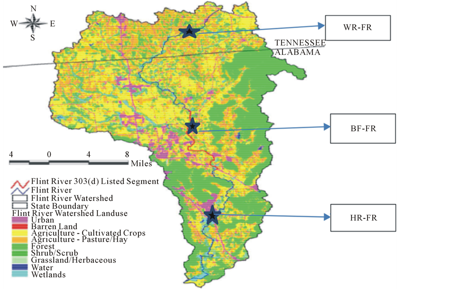
Table 1. Showing the Flint Creek (FC) and Flint River (FR) Geographic Point Coordinates (GIS).
FR (codes: WR-FR = Winchester Road, BF-FR = Briar Fork, HR-FR = Hobbs Road); FC (Codes: RB-FC = Red Bank, MB-FC = Means Bridge, VB-FC = Vaughn Bridge).
 (a)
(a)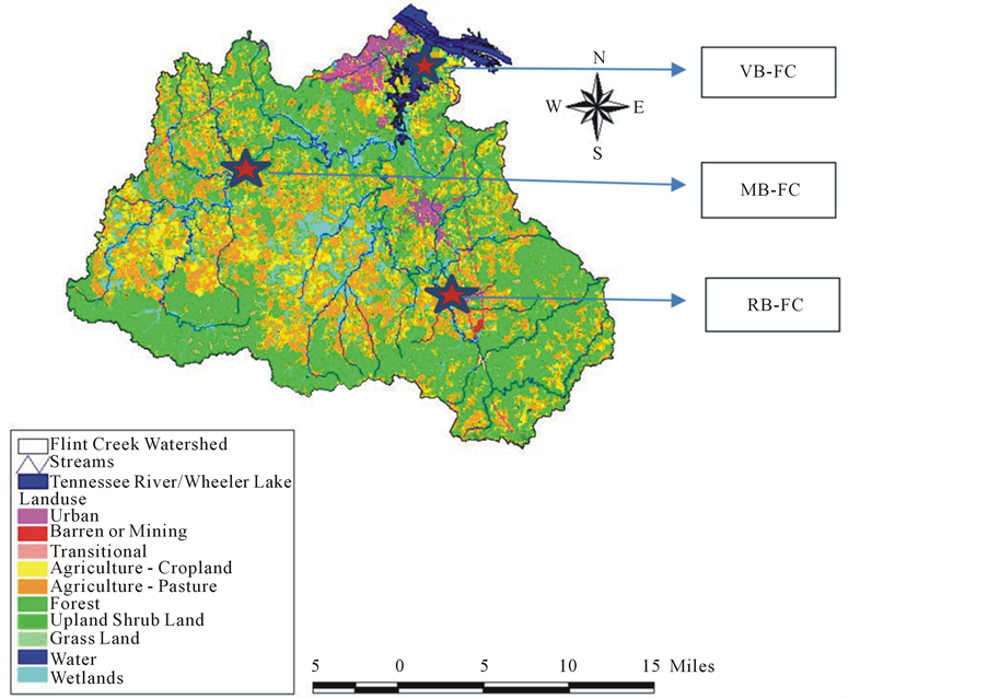 (b)
(b)
Figure 1. (a) Sampling sites: at the Flint River Watershed (Okweye, P., PhD dissertation, 2009); (b) Sampling sites: at the Flint Creek Watershed (Okweye, P., PhD dissertation, 2009).
Table 2. Soil Types for the FC and FR Watersheds (Courtesy: Joe Gardinski, NRCS).
2.2. Sample collection
Soil/sediment samples were collected in winter/spring 2014 from six sites (WR-FR, BF-FR, HR-FR, RB-FC, MB-FC, and VB-FC) as shown in Figure 1(a); Figure 1(b) and Table 1. Samples were transferred into sampling bags and placed in a cooler at 4˚C, and then transported to Alabama A&M University laboratories for storage. About 1 kg of sample was obtained from each site and air dried before analysis. All the sampling locations were recorded with a GPS. Most of the samples were fine-grained clay and silt, and passed through a 1 mm metal sieve.
The soil/sediment sampling locations for each site included: 1) an in-stream/Depositional area, 2) a Bank-side, and 3) an Upland in riparian zone. At each location, five samples were collected, composited, and well-mixed to obtain a representative sample (Figure 2). A stainless steel soil probe was used to collect soils from the banks and upland areas, and a 250-cm pole sediment sampler―Pakar [5] was used for collecting sediments from in- stream/depositional areas across the upper, middle, and lower sections of the streams, covering a distance of ~110 km. The sediment sampling was carried out in low flow conditions because trace metal concentrations tend to be highest during this period as metals accumulate in the sediments from water. Under high water discharge, erosion of riverbeds takes place. According to the UNEP/WHO [6] , following peak discharge, the concentrations of metals in bed sediments increase as the water flow again decreases. A total of seventy-two (72) soil/ sediment samples were collected from the watersheds. In the laboratory, samples were stored in the freezer until they were processed and analyzed. In-situ measurements for physical and chemical characteristics of water and soil properties were conducted at the sites with a 6600 Extended Deployment System (EDS).
2.3. Analytical methods
USEPA Method 3050B [7] was used for the digestion of heavy metals in soil/sediment samples at the Environmental Testing and Consulting (ETC) laboratories in Memphis, Tennessee. This method is suitable for hot block digestion of soil, sediment, and waste samples and for analysis by inductively coupled plasma optical emission/atomic emission spectrometry (ICP-OES/AES). A 1.0 g subsample of each sample was digested in nitric acid and hydrogen peroxide. The digestate was then further refluxed with hydrochloric acid. High-tech instrument ICP-AES, with SW-846 USEPA method 6010B, was used for the elemental determination. The USEPA standard sediment samples were used to monitor the analyses. Al, Fe, Mn, and Pb was measured by inductively coupled plasma optical emission spectrometry (ICP-OES, Optima 2000DV; Perkin Elmer, Waltham, MA, USA; detection limit 0.001 - 0.030 mg/L) and inductively coupled plasma-mass spectrometry (ICP-MS, 7500a; Agilent Technologies, Santa Clara, CA, USA; detection limit 0.015 - 0.120 mg/L) was used for the analysis for Arsenic (As). Laboratory quality control consisted of analysis of sediment reference material (GBW 07302- 07312a; National Institute of Standard and Technology, MD, USA) and triplicate samples were used. The results were consistent with the reference values, and the differences were generally within 10% (most were within 5%).
The recoveries all fell within the range of 90% - 110%, and the relative standard deviation was less than 5%. All The reagents used for the analysis were AR grade and double distilled water was used for preparation of solutions. The analyzing laboratory - ETC asserted that the results from the average values of the concentrations of the elements detected by both ICP-OES/AES (Al, Fe, Mn, and Pb) and ICP-MS (As) were consistent. The quality control in this study was similar to that used in a previous study in the area [3] . ICP-MS was used for arsenic
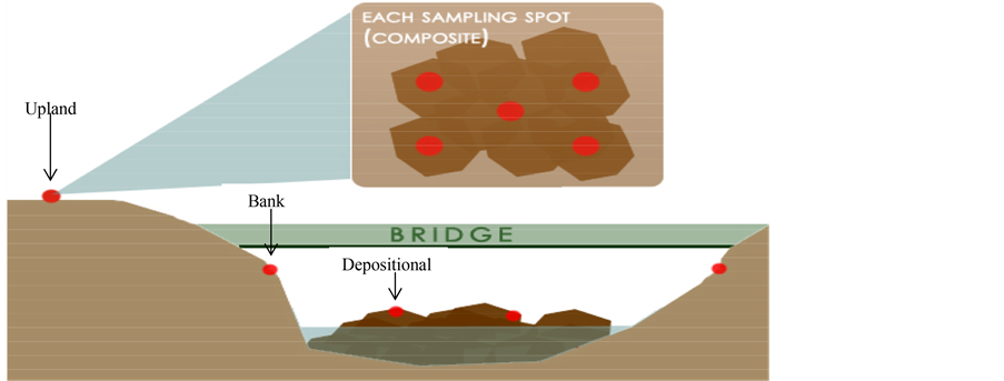
Figure 2. Diagram of a sampling site and spots sampled.
analysis in this research because it offers multi-element detection limits below parts per billion (ppb; 10−9), sometimes down to parts per trillion (ppt; 10−12), and can give a rapid throughput of samples [8] -[10] .
2.4. Soil/Sediment Texture Analysis
The relative proportions of sand (particle size between 0.06 and 2 mm), silt (0.002 and 0.06 mm), and clay (< 0.002 mm) in the soil/sediment samples were determined by means of the classical sieve-pipette technique. This method involves sieving of the sand fractions and pipette extraction of the clay fractions using settling tubes. The results may be due to the soil types of the various sites (Table 2)
2.5. Data Analysis
3. Results and Discussion
All the locations in both FC and FR watersheds had high percentages of the fine particle (clay) size and low percentages of the coarse (sand) particle sizes (Table 3). The samples were probably located at sites where there were low currents in the rivers during run-off periods and where only the fine sizes of the sediment were deposited and retained. Texture was not uniformly distributed along the sites; this may be due to soil types (Table 2); FC locations had lower percentages of silt particle sizes than FR locations (Table 3).
Table 3. Spatial distribution of particle sizes measured in depositional and upland areas of the FC and FR watersheds.
D = dispositional area, U = upland area.
Particle Size Effect
Table 4. Coefficient of determination (r2), SAS proc corr.
(a) +ve and −ve: positive and negative correlations: [*(orange), and **(red): significant and highly significant at 0.01 and 0.05 levels]; (b) ns: not significant.
Studies have shown that one of the most significant parameters influencing total recoverable metal levels in sediments is particle dimension [1] . Bio-available sediment-bound metals such as Al, Fe, Mn, As, and Pb, depend to a significant extent on the particle size fraction with which a metal is associated. This study showed that the highest concentrations of metals were associated with fine grained sediment particles. Table 4 shows that Fe was significant, but negative correlations with sand, and positive but highly significant correlations with silt. Arsenic (As) was highly significant. There were positive correlations with silt and negative but significant correlations with clay.
In the FC and the FR watersheds, the spatial distribution of the particle size of sediments was coarser from upland to depositional (Table 3). The results showed that texture played a controlling role on the concentrations and their spatial distribution. Principal component analysis and cluster analysis were carried out based on the particle sizes of the sediments, and the samples were classified into three fractions: sand, silt and clay. Significant differences among the element concentrations in the three groups were observed, and the concentrations of the elements in each group were reported in this study (Table 5). Most of the elements had their highest concentrations at the sites with high, fine particle (silt and clay) samples; in comparison with the sand samples, with clay minerals possibly playing an important role. The heavy metals being mainly present in the clay-silt particles with particle sizes less than 63 μm (<0.06 mm), may be due to the increase in specific surface properties of this fraction. An upland to depositional spatial variation of element concentrations in the sediments was observed. This is in line with the spatial distribution of the particle size and may be due to the water hydrological dynamics in the rivers.
3.1. Correlation Coefficients
The Factor Analysis for the data was developed in three stages:
Table 5. Average of heavy metals in combined soil/sediment samples.
1) A correlation matrix was generated for all the variables,
2) Factors were extracted from the correlation matrix based on the correlation coefficients of the variables; and
3) The factors were rotated in order to maximize the relationship between the variables and some of the factors.
For a better understanding of the relationships between the heavy metal log transformed concentrations and particle sizes, correlation coefficients were calculated and listed in Table 6(a) and Table 6(b).
The Pearson correlation coefficient was used to determine the linear association between two variables, using data that was transformed and normally distributed. The Fe and As elements in Table 7(a) had negative correlations with the sand (>0.06 mm). With the exception of Al, all the other elements had moderate to significantly positive correlations with silt (<0.06 mm) and clay fractions of <0.02 mm of the sediments. Mn is the only element with significantly positive correlations with the finest grained sizes of <0.02 - 0.05 mm, and sand fractions (>0.06 mm).
All the elements in Table 7(b) have significantly positive correlations with the silt (<0.06 mm) and sand fractions (>0.06 mm) of the sediments. Mn was the only element with significantly positive correlations with the finest particle sizes of <0.02 mm. However, Al, Fe, As, and Pb had moderately negative correlations with the coarse particle sizes of >0.06 mm. Therefore, all the elements in this study appear to be influenced by the particle size effect in some manner.
3.2. Sample Classification
Cluster Analyses was applied for sample classification based on the particle sizes and elements detected. In addition, PCA and correlations were applied to reduce the variables between the particle sizes and the elements; factor analysis uses the correlation matrix to determine which sets of variables cluster together. Before the multivariate analysis, tests were conducted to test the normality of the datasets. All of the elements and the particle sizes passed the normality tests at the significance level of P ≤ 0.05. Therefore, all the raw data (real observed data points) were used without any transformation for the following multivariate analyses. The matrix of correlation coefficients and their significance levels are shown in Table 8(a) through Table 9(b).
According to Hatcher, L. [14] , confirmatory factor analysis (CFA) is a statistical approach used to examine the internal reliability of a measure; to investigate the theoretical constructs, or factors, that might be represented
(a) (b)
Table 6. (a) Pearson correlation coefficients for depositional areas; (b) Pearson correlation coefficients (upland−reference area).
*= Correlation is significant at the 0.05 level (2-tailed); **= Correlation is significant at the 0.01 level (2-tailed).
(a) (b)
Table 7. (a) Correlation matrix for depositional areas; (b) Correlation matrix for upland areas.
(a) (b)
Table 8. (a) Component score coefficient matrix for depositional area; (b) Component score coefficient matrix for upland area.
Extraction Method: Principal Component Analysis; Rotation Method: Varimax with Kaiser Normalization.
(a) (b)
Table 9. (a) Total variance explained (Depositional); (b) Total variance explained (Upland).
Extraction Method: PCA.
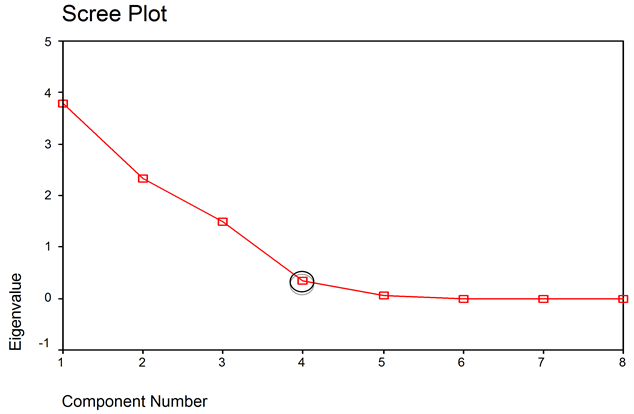
by a set of variables, such as, given in this study (Al, Fe, Mn, As, Pb, sand, silt, and clay) and to assess the quality of individual variables. According to Cattell, R.B. [15] , researchers typically use maximum likelihood in the CFA model to estimate factor loadings, and the most common approach to deciding the number of factors to generate a scree plot. The scree plot is a two dimensional graph with factors on the x-axis and eigenvalues on the y-axis. The scree plot was used to help determine the number of factors to keep in the analysis. Theoretically, an eight-item variable will have eight possible underlying factors, and each factor will have an eigenvalue that indicates the amount of variation in the items accounted for by each factor. It should be noted that this approach to selecting the number of factors involved a certain amount of subjective judgment. From the scree plot (Figure 3(a) and Figure 3(b)), there were three underlying factors for each plot (components 3, 4, 5 for depositional and components and 1, 2, and 3 for upland area). It is believed that the remaining of factors were due to unknown error variation.
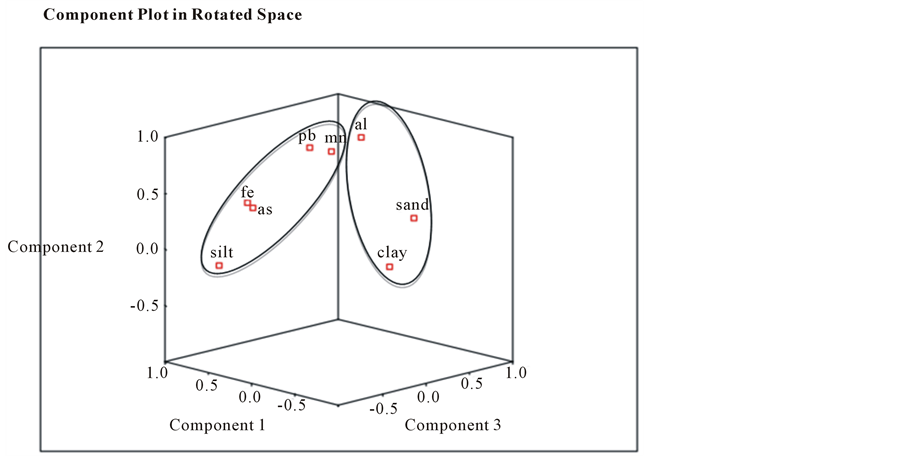
The component plot in rotated space shows the first three principal components (PCs) for the depositional area (Figure 4(a)), and the upland area (Figure 4(b)). The first three PCs may reveal a clearer explanation of the particle-size and element factor controlling the distribution and accumulation of the metals and particle sizes. The significant relationships between the particle-size variables and the elemental components were presented
 (a)
(a)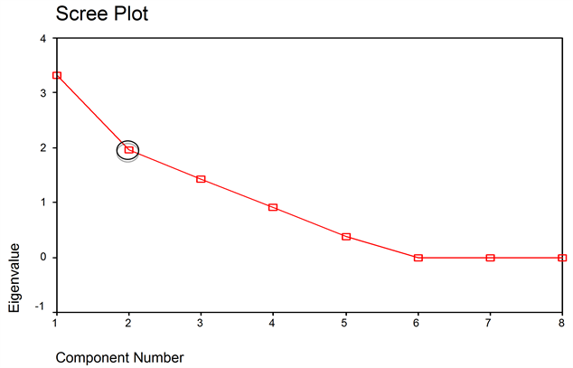 (b)
(b)
Figure 3. (a) Scree Plot for the Depositional Area; (b) Scree Plot for the Upland Area.
 (a)
(a)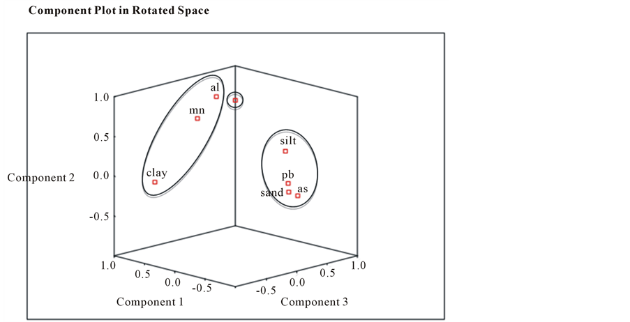 (b)
(b)
Figure 4. (a) FA in Rotated Depositional Space; (b) FA in Rotated Upland Space.
by using FA as the indicators. The first three PCs in the depositional area accounted for 95.12%, and the upland area accounted for 83.84% of the total data variance explained. They were selected for subsequent graphical displays and analysis. Figure 4(a) and Figure 4(b) show the PC loadings of the particle sizes and the elements on the first three principal components. In the depositional area the fine particle sizes of <0.05 and <0.02 mm had low negative loadings of PC2, and the coarse sizes of >0.06 mm had high positive loadings of PC3. In upland area the fine particle sizes of <0.05 mm had low negative loadings of PC2, and the coarse sizes of >0.06 mm had low negative loadings of PC3, but silt <0.02 mm had a high positive loadings in PC3. The summary scores on the two PCs are shown in Figure 6(a) and Figure 6(b). It can be seen that many samples were located on both sides of the positive and negative values of PC2, and some samples were located at the side of high values of PC3 and no values in PC1. It is expected that the multi-element concentrations among the three PC loading of samples should be different. Since the initial solution was obtained, the loadings are rotated. Rotation is a way of maximizing high loadings and minimizing low loadings so that the simplest possible structure is achieved.
For this study, oblique rotation was used because it derives factor loadings based on the assumption that the factors were correlated. This was the case for these measures (variables). The oblique rotation gave the correlation between the factors in addition to the loadings (See Table 10).
3.3. Cluster Analysis for Upland Area
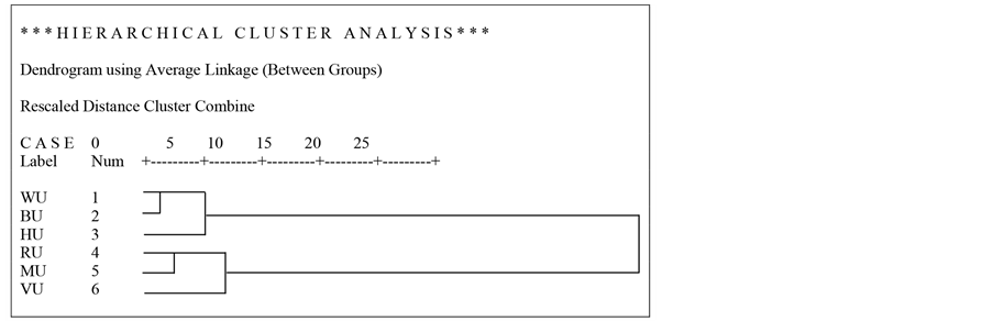
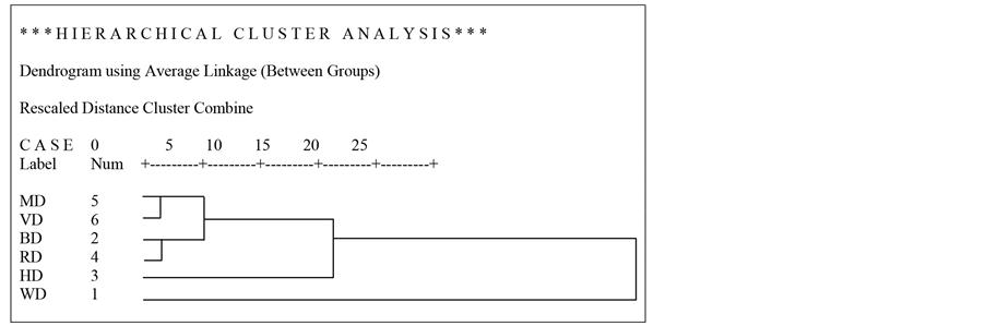
Table 11, cluster membership displays the single solution cluster (between-groups linkage model option) to which each variable was assigned. Each stage (site) was assigned one predominant variable. The icicle plot, in Table 12, displays vertical information about how variables were combined into clusters at each iteration of the analysis. The agglomeration scheduled hierarchical CA identified relatively homogeneous groups of variables based on selected characteristics. It shows that Al was dominant in WR-FR; Fe in BF-FR; Mn in HR-FR; As in RB-FC; Pb in MB-FC, and all the metals were clustered in VB-FCs site sediments of upland areas.
The dendrograms plot below used the nearest neighbor model to assess the cohesiveness of the clusters formed. It shows that Mn, Pb, and As were clustered in all the particle sizes as shown, and the cluster of Al and Fe were observed mainly in the clay proportion of the sediments (see Figure 5(a) and Figure 5(b)).
Table 10. Summary of the Loadings from the oblique rotations for depositional and upland areas of the fc and FR watersheds.
Table 11. Cluster membership.
Table 12. Verticle icicle.
 (a)
(a)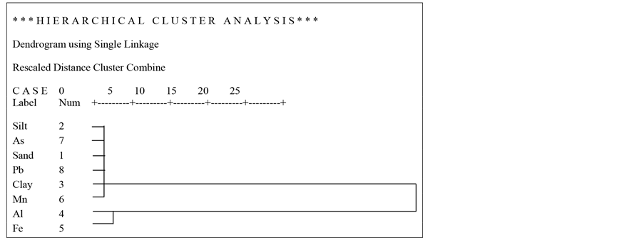 (b)
(b)
Figure 5. (a) Dendrogram using average linkage (between groups); (b) Den- drogram using single linkage.
3.4. Cluster Analysis for Depositional Area
Table 13(a) Cluster membership, shows the single solution cluster (between-groups linkage model option) also to which each variable is assigned. Here each depositional site on the watershed was assigned only one predominant variable. The icicle plot, in Table 13(b), displayed vertical information about how variables are combined into clusters at each iteration of the analysis. The agglomeration scheduled hierarchical cluster analysis identified relatively homogeneous groups of variables based on selected characteristics. It showed that MB-FC and VB-FC had similar clustering, BF-FR and RBFC had similar clustering, and that HR-FR and WF-FR had different clustering for all the metals in site sediments of depositional area.
The dendrograms plots below used the (nearest neighbor model) to assess the cohesiveness of the clusters formed. It shows that As and Pb were clustered in all the particle sizes as shown, and Mn was clustered in clay, but Al and Fe cluster were observed mainly in the clay proportion of the sediments (see Figure 6(a) and Figure 6(b)).
3.5. Concentrations
The arithmetic means of the particle size compositions and element concentrations in all the sediment samples consisting of sand, silt, and clay were calculated, and listed in the tables below. The depositional samples, as hypothesized, had high percentages of the grain sizes <0.02 mm. The sand samples, on the other hand, mainly consisted of the coarse sizes >0.1 and 0.05 - 0.1 mm. All of the particle-size groups were relatively evenly distributed in the silt-clay samples. Most of the elements under study were elevated in the clay samples, and depleted in the silt samples. Concentrations of the elements in the silt-clay samples were between the clay and silt samples.
 (a)
(a)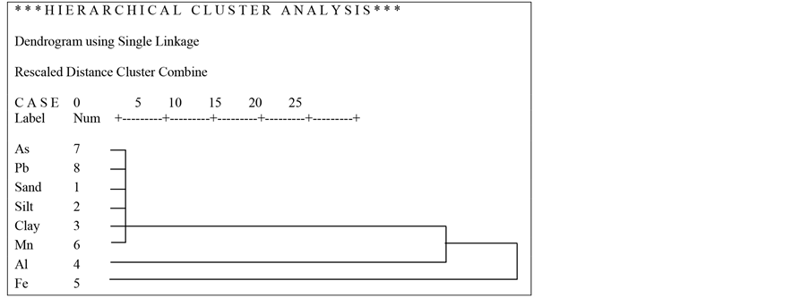 (b)
(b)
Figure 6. (a) Dendrogram using average linkage (Between groups); (b) Den- drogram using single linkage.
(a) (b)
Table 13. (a) Cluster membership; (b) Verticle icicle.
Table 14(a) and Table 14(b) list the concentrations of the five elements Al, Fe, Mn, Pb, and As. Most of the element concentrations of Al, Fe, Mn, As and Pb were highest in the clay samples. However, Al in depositional and As in upland were elevated in the sand samples. The particle size effect on total metals has been widely studied. Clay minerals and other fine particle minerals play an important role in trapping and holding total metals. In this study, the same conclusion for the total metals was reached. The PC loadings of the particle sizes on the second and third PCs contain all of the Al, Fe, Mn, As and Pb. Further studies on the relationships between multi-element composition, and particle sizes are needed.
4. Conclusions
Sediments along rivers have different textures, as shown in the samples studied in these two watersheds, depending on whether the stream moves quickly or slowly [16] [17] . Fast-moving water leaves gravel, rocks, and sand. Without storm events, the FC and the FR have slow-moving water and tend to leave fine textured material (clay and silt) when sediments in the water settle out. The study evaluated spatial and compositional patterns in the FC and FR sediment contaminant data using the multivariate techniques―principal components analysis (PCA) and
(a) (b)
Table 14. (a) Soil texture and heavy metals in depositional sediments; (b) Soil texture and heavy metals in upland soil samples. (SAS proc glm with Duncan’s Multiple Range Test) (a, b, c, d = Average Means (Duncan Grouping) with the same letter are not significantly Different).
cluster analysis (CA). With the aid of PC and CA, the sediments from these watersheds were classified based on their texture into three fractions: sand, silt and clay. Significant differences were observed among the concentrations of the elements in the categories. Most of the elements detected were enriched in the fine-particle samples, where clay minerals were an important constituent [3] . On the other hand, elevated concentrations of Al and As were observed in the coarse (sand) samples. This may imply that the Al and As were present in the parent materials that weathered to sand. PCA indicated association among all heavy metals determined in the environmental matrices (soil/sediment) analyzed, revealing that their high concentrations were due to the discharge of liquid wastes to the FC and FR watersheds. Interestingly, some of the wastewater from the Decatur plant enters the river untreated [18] . According to Gray [19] , sewage treatment removes less than 100% of the metals from wastewater, so untreated wastewaters can be an important source of metals such as the ones analyzed in this study. Further, CA correlated all sampling sites impacted by contamination resulting from non-point sources, municipal wastes, sewages, and other sources. Metal concentrations from this study were higher than the USEPA’s MCL or background concentration values for Al, Fe, Mn, As and Pb. This indicated that there was metal pollution at all the sampling sites. Significant relationships from the Pearson’s correlation were also supported by the results of the statistical methods (PCA and CA) used.
In summary, contaminants displayed distinct groupings (elements with similar properties) and spatial patterns; and relationships between particle size factors and chemical contaminant concentrations were explained in part with the multivariate statistical approaches. However, this multivariate statistical approach was as effective as simple correlation for this study, where contaminant concentrations were relatively high and correlation patterns were strong. In addition, the study refuted the null hypotheses. There was enough evidence from the overall results of the study to support the theoretical notion that particle size distribution and sampling location influenced the level of heavy metal concentration within the watersheds. These results provide a framework for interpreting heavy metal distribution and sediment toxicity in biological communities at these watersheds.
Acknowledgements
We would like to acknowledge Alabama A&M University Interdisciplinary Center for Health Sciences and Health Disparities in the College of Engineering, Technology and Physical Sciences with funding provided through the Evans-Allen Grant, administered by the College of Agricultural, Life and Natural Sciences (CALNS).
Cite this paper
Paul S.Okweye,Karnita G.Garner,Anthony S.Overton,Elica M.Moss, (2016) Factor-Cluster Analysis and Effect of Particle Size on Total Recoverable Metal Concentration in Sediments of the Lower Tennessee River Basin. Computational Water, Energy, and Environmental Engineering,05,10-26. doi: 10.4236/cweee.2016.51002
References
- 1. Greany, K.M. (2005) An Assessment of Heavy Metal Contamination in the Marine Sediments of Las Perlas Archipelago, Gulf of Panama. Master of Science Thesis, Heriot-Watt University, Edinburgh.
- 2. Pekey, H.P., Karakas, S., Ayberk, L., Tolun, L. and Bakoglu, M. (2006) Ecological Risk Assessment Using Trace Elements from Surface Sediments of Izmit Bay (Northeastern Marmara Sea) Turkey. Marine Pollution Bulletin, 48, 9-10, 946-953.
- 3. Okweye, P., Tsegaye, T.D. and Garner. K.F. (2007) Distribution of Heavy Metals in Surface Water of the Wheeler Lake Basin in Northern Alabama. Journal of Environmental Monitoring and Restoration, 33, 91-100.
- 4. Phillips, C.R. (2007) Bulletin of the Southern California Academy of Sciences, 106, 163-178, E Article 1.
- 5. Okweye, P. and Garner, K.F. (2009) Sediment Sampler (Patent Pending).
- 6. United Nations Environment Program and the World Health Organization (1996) Sediment Measurements. Water Quality Monitoring—A Practical Guide to the Design and Implementation of Freshwater Quality Studies and Monitoring Programs Edited by Jamie Bartram and Richard Balance.
- 7. U.S. Environmental Agency (USEPA) (1994) 822-R-94-001. Drinking Water Regulations and Health Advisories. EPA’s Toxics Release Inventory, 1-3.
- 8. Date, A.R. and Gray, A.L. (1989) Applications of Inductively Coupled Plasma Source Mass Spectrometry: Blackie, Glasgow.
- 9. Platzner, I.T. (1997) Modern Isotope Ratio Mass Spectrometry. Chemical Analysis, 145, 187-189.
- 10. Kennett, D.J., Neff, H., Glascock, M.D. and Mason, A.Z. (2001) A Geochemical Revolution: Inductively Coupled Plasma Mass Spectrometry. The Archaeological Record, 1, 22-26.
- 11. Grimm, L.G. and Yarnold, P.R. (2000) Introduction to Multivariate Statistics. In: Grimm, L.G. and Yarnold, P.R., Eds., Reading and Understanding More Multivariate Statistics, American Psychological Association, Washington DC, 3-21.
- 12. SCB (2007) Bulletin of the Southern California Academy of Sciences, 106, 163-178, E Article 1.
- 13. Phillips, C.R. (2007) Bulletin of the Southern California Academy of Sciences, 106, 163-178, E Article 1.
- 14. Hatcher, L. (1994) A Step-by-Step Approach to Using the SAS® System for Factor Analysis and Structural Equation Modeling. SAS Institute Inc, Cary.
- 15. Cattell, R.B. (1966) The Scree Test for the Number of Factors. Multivariate Behavioral Research, 1, 245-276.
http://dx.doi.org/10.1207/s15327906mbr0102_10 - 16. Alagarsamy, R. (2006) Distribution and Seasonal Variation of Trace Metals in Surface Sediments of the Mandovi Estuary West Coast of India. Estuarine, Coastal and Shelf Science, 67, 333-339.
http://dx.doi.org/10.1016/j.ecss.2005.11.023 - 17. Jonathan, M.P., Ram-Mohan, V. and Srinivasalu, S. (2004) Geochemical Variations of Major and Trace Elements in Recent Sediments, off the Gulf of Mannar, Southeast Coast of India. Environmental Geology, 45, 466-480.
http://dx.doi.org/10.1007/s00254-003-0898-7 - 18. (2008) ADEM Files Suit against Hanceville Water Board. Huntsville Times, 15 June 2008, p. A20.
- 19. Gray, D. (2004) Doing Research in the Real World. SAGE Publications, Various Paginations.
NOTES

*Corresponding author.