Computational Water, Energy, and Environmental Engineering
Vol.3 No.1(2014), Article ID:40666,14 pages DOI:10.4236/cweee.2014.31002
A New Space-Time CE/SE Numerical Tracking of Contaminant Transport in Fractured Stratified Geologic Profiles
Department of Systems Engineering, University of Lagos, Lagos, Nigeria
Email: tfashanu@unilag.edu.ng, vosolunloyo@hotmail.com
Received October 11, 2013; revised November 11, 2013; accepted November 18, 2013
ABSTRACT
To date, efficient numerical simulation of contaminant transport in geologic porous media is challenged by parametric jumps resulting from stratification and the use of ideal initial/boundary conditions. Thus, to resolve some contaminant hydrology problems, this work presents the development of the Space-Time Conservation Element/Solution Element (CE/SE) scheme for advection-dispersion-reaction a-d-r transport in geologic media. The CE/SE method derives from the native form of Gauss conservation law. Therefore, it is able to effectively handle non-trivial discontinuities that may exist within the problem domain. In freshwater aquifer, stratification and other parametric jumps are examples of such discontinuity. To simulate the Nigerian experience of nitrate pollution of freshwater aquifers; the a-d-r contaminant transport model is herein solved under a time periodic nitrate fertilizer loading condition on farmlands. Results show that this approach is able to recover the wellknown field pattern of nitrate profiles under farmlands. Cyclic loading impacts more on the dispersivity of an aquifer. Hence, dispersion coefficient modulates the response of aquifers to loading frequency. However, aquifers with conductivity less than 10−6 m/day are almost insensitive to periodic loads. The CE/SE method is able to sense slight (i.e. order of 10−3) variation in hydrological parameters. Also, CE/SE computes contaminant concentration and its flux simultaneously. Thus, it facilitates a better understanding of some reported phenomena such as contaminant accumulation and localized reverse transport at the interface between fracture and matrix in geologic medium. Clearly, CE/SE is an efficient and admissible tool into the family of numerical methods available for tracking contaminant transport in porous media.
Keywords:CE/SE Scheme; Contaminant Tracking; Freshwater Aquifer; Periodic Loading; Stratification
1. Introduction
The Space-Time Conservation Element/Solution Element (CE/SE) method is gradually emerging as a reliable tool for tackling some problems in engineering and mathematical physics. In particular, it has been used to resolve some challenging problems in aero-acoustics and related shock flows. These include the shock tube and multicomponent combustion problems as treated in [1]. However, at the other end of this class of problems are some issues in environmental systems. For example, in percolation problem, process rates are slow and sometimes of geological time scale. To assess the efficacy of CE/SE method in this regime, we look at the transport of contaminants through geological profile. Although, there are many analytic, semi-analytic and numerical methods for modeling and simulation in this regime, to date, none of these methods is able to completely capture all the intricate features of the actual flow pattern as met in practice.
In approach, two basic concepts, namely; the percolation and hydro dispersive schemes are generally used to model transport of contaminants through geologic systems. However, in recent time, attempts have been made to hybridize these models. For example, [2] is an innovative work in this regard. The microscopic approach considers transport on the basis of individual pores in the medium. Therefore it models the boundaries of an aquifer as an infinite network of interconnected pores of various sizes. This represents a skeletal conglomerate of solid element having variable porosity and permeability.
On the other hand, the macroscopic framework of contaminant transport in geologic systems differentiates between coordinated and uncoordinated pore spaces. The coordinated pore spaces determine some macroscopic properties of the aquifer e.g. conductivity and permeability. However, uncoordinated pore spaces determine other properties such as storativity, adsorption and retardation. Under certain flow condition, an additional term is used to model geo-chemical reaction or physical transformation. For example, [3] is a recent formulation of hydrodispersive scheme that pays special attention to geo-chemical reaction. To simplify analysis, the macroscopic model resolves contaminant flow in a geological medium into two major zones; namely the momentum transport zone, where fluid flow is large and a region of small fluid flow dominated by other transport processes. The overall process is usually described by the parabolic or hyperbolic partial differential equations in two or higher spatial dimensions. In principle, this equation is an expression of conservation laws. However, in an ideal situation, conservation laws are best expressed as integral equations. This is more important when the domain of the problem is discontinuous. However, most existing works in this field are based on differential equations. The underlying assumption is that the domain is smooth. In natural groundwater reservoirs, this assumption does not hold. Real aquifers are known to consist of various geological formations with sharp differences in hydrological properties.
Traditionally, the Finite Difference, Finite Elements and Finite Volume methods are the well-known numerical tools that are used to solve contaminant transport problems. These tools take on the differential form of the conservation laws. Hence, they dissipate flux in the neighborhood of discontinuity. In such regions, the computational grid is usually refined to minimize flux dissipation. However, the need to satisfy the Courant, Friedrich, and Lewy (CFL) stability conditions sometimes overshoots the cost of this strategy. In the case of the FD, some robust schemes have been recently developed with enhanced flux conservation, stability and accuracy features. These schemes are built on the concepts of Total Variation Diminishing (TVD) and localized flux conservation, [4]. However, TVD schemes are also computationally expensive.
On the other hand, the Finite Element Method (FEM) obtains an approximate solution of the transport equation using the trial solution approach. The individual steps involved in FEM analysis are quite simple. However, the method becomes numerically tedious especially at the point where the elementary solutions are assembled to build the global solution. According to [5], at this stage, FEM has a tendency to divorce the modeler from the physics of the problem. In addition, for the trial solution to be adequate in regions of rapid changes, higher order basis functions or very fine grids of complex geometry are usually required. This inflates computational cost. Furthermore, [6] observed that FEM hardly evaluates dependent variable at the borderline of two adjacent elements. Hence, FEM may not be best suited for problems with non-trivial discontinuities. Although FEM solves some form of integral equations, these do not derive from the original form of conservation law. They are equivalence of the differential form of conservation law under Reynolds transport theorem. Other limitations of FEM in this regime are reiterated in [7]. Despite these shortcomings; FEM remains an efficient numerical tool in computational physics, structural mechanics and environmental research. For example, using exponential element approach, [8] presents a novel FEM analysis of multiple porosity contaminant transport in porous media. However, most other works are based on available commercial FEM packages for contaminant tracking in geologic profiles.
In addition to domain discontinuity, there are instances in contaminant hydrology problems when the model equation alternates between parabolic and hyperbolic states. This depends on the instantaneous order of magnitude of the advection and diffusion speeds. This instability in physics often leads to severe numerical oscillations. In such cases, standard numerical schemes that are built on the differential forms of conservation law are known to experience some difficulties. To handle such difficulties, extensive studies have been carried out either to customize standard methods, or design new ones. However, most of the emerging schemes are designed to address specific types of interface, or resolve definite numerical problems. Notable on this list is the Euler-Lagrangian based schemes. They include localized adjoint method and Eulerian-Lagrangian localized adjoint method developed in [9]. Although, the adjoint method and its derivatives are able to optimize flux dissipation, they do not enforce mass conservation and are deficient in ability to handle general boundary conditions.
Spatial and temporal scale-effects are additional difficulties with numerical simulation of contaminant transport in geologic media. They induce errors in contaminants profiles in aquifers. In a finite element analysis, [10] noted that scale effects are amplified at the interface between two strata even when the axis of flow is parallel to stratification. To handle scale-effect, [11] developed a stochastic mixed finite element technique that coarsens the flow equation in space. This is followed by piecewise parameter up-scaling using adaptive sparse grid collocation method. Clearly, the method does not completely account for parametric jumps that are common in real aquifers. On the same note, [12] used a strategic porous medium with high fracture frequency to present a numerical solution for colloid facilitated contaminant transport in aquifers. This minimized scale effect, but the approach is constrained by the high cost of computing.
For the foregoing reasons, we herein present the Space-Time Conservation Element/Solution Element numerical method as an efficient tool for contaminant tracking in fractured porous media. The CE/SE method is a collection of innovative numerical tools originated by [13,14] for solving conservation laws. It was developed from a perspective that is quite different in concept and methodology from traditional numerical schemes. Its development was motivated by the desire to build a general and coherent numerical framework that avoids many of the limitations of traditional numerical methods.
Rather than the differential form of the conservation laws, the CE/SE method derives its solution from the native Gauss integral form of the conservation law. As a result, local and global flux conservation is intrinsic to CE/SE formulations. Therefore, it is able to overcome most limitations encountered by numerical schemes that are built on the differential form of conservation laws. In effect, CE/SE solutions are naturally compliant with the physical model. Like other numerical schemes, the CE/ SE method uses an approximating function i.e. the Taylor series to describe numerical approximation of the exact solution on a computational mesh. The CE/SE mesh consists of Conservation Elements (CE) and Solution Elements (SE). A CE is a small region in two-dimensional Euclidean space E2, within which flux conservation is enforced. This ensures global flux conservation. On the other hand, a SE is another small region in E2 within which unknown variables are approximated.
2. Transport Equations
In this work, we consider the hydro dispersive scheme of contaminant transport in two dimensions. Thus, three transport processes namely advection, dispersion and reaction are combined to describe the concentration profile i.e. C(y,z,t) of an aqueous contaminant in natural freshwater aquifer. The effects of sorption and retardation are also considered to give the governing differential equation as:
 (1)
(1)
where
 (2a)
(2a)
 (2b)
(2b)
Here, uz and uy are the longitudinal and transverse velocities of fluid. Similarly, Dz and Dy are the corresponding dispersion coefficients, while Ry and Rz are the coefficients of retardation of the contaminant along y and z directions respectively. Ã is the rate constant of the attendant geo-chemical and allied reactions. ay and az are coefficients of dispersivity, while  is the diffusivity index of the medium.
2.1. The Physical Model
Next we simplify Equation (1) by using the dual porosity concept to delineate contaminant pathways into two regions. The momentum transport zone called the channel. Flow in the channel is coupled with transport processes such as sorption, diffusion, and reaction in the adjoining matrix. Thus, using some simplifying assumptions as detailed in [15], an iconic model for this system of flow is illustrated as in Figure 1.
We consider channels of thickness D, bounded by vertical lines at −D and the origin. The centerline of the channel is at −D/2. The matrix separating two channels proceeds from the origin along the horizontal axis to 2x. Therefore, the matrix centerline is at y = x. Consequently, for this flow system, the equivalence of Equation (1) for transport in the channel and matrix is given by Equations (3) and (4) respectively.
 (3)
(3)
where C(0,z,t) = C(y,z,t) y = 0
 (4a)
(4a)
with
 (4b)
(4b)
2.2. Model Simplification
For further simplification, we normalize flow parameters in Equations (3) and (4) with their corresponding scale factors. Then we group the resulting parameters into standardized dimensionless forms. This is followed by order of magnitude analysis following the approach of
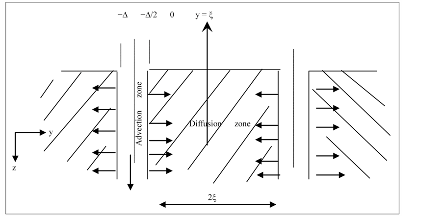
Figure 1. Flow geometry of contaminant motion in fractured porous medium.
[15,16]. Hence, Equations (3) and (4) are reduced to Equations (5) and (6) respectively.
 (5)
(5)
 (6)
(6)
Equation (6) derives from Equation (4) under the assumption that the Peclet number only applies to the channel. In this case, the reaction term is treated as a first order geochemical reaction. In addition, the following non-dimensional variables apply

2.3. Contaminant Loading and Boundary Conditions
Next, we consider the boundary and initial conditions needed to complement Equations (5) and (6). Here, we attempt to model the Nigerian experience of nitrate pollution of groundwater resources. Thus, we introduce a realistic and coherent boundary condition for the associated groundwater pollution problem. Precisely, we simulate what obtains in normal agricultural practice. In this case, seasonal loading of inorganic fertilizer with an arbitrary nitrate concentration Co is normally applied on topsoil. The surface behavior of the applied nitrate fertilizer is herein modeled as an integral Dirichelet/Neumann condition. This gives an exponentially decaying function of the form Co . The function accounts for the progressive decay of the contaminant on topsoil as a result of some physico-chemical processes. With repeated seasonal (i.e. periodic) applications, the corresponding nitrate profile on topsoil can be represented as shown in Figure 2.
Here, β is the rate of disappearance of applied fertilizer on the soil surface. This may be due to percolation, evaporation, runoff etc. n is the number of cycles of fertilizer applications. On extension, the contaminant loading profile described above has widespread practical applications. With slight modification, it can be used to handle various types of physical loading conditions that are of interest to contaminant hydrologists and environmentalists. To be sure, the periodic, exponentially decaying function truly models actual physical conditions better than the impulsive, uniform and step function loadings that are well considered in literature. For instance, a leaking canister of toxic waste in a geological repository can be considered as having periodic effect on the surrounding aquifer, if for instance a similar canister has leaked in the region in the past or will most probably leak in the future. Such periodic loading profiles act to alter the hydrological properties of the aquifer and the initial concentration of the latest spill.
Our analysis is now reduced to solving simultaneous partial differential equations posed in Equations (5) and (6) to track the breakthrough curves of the contaminants in time and depth of an aquifer, under the normalized boundary condition:
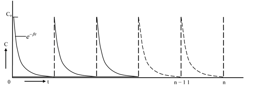
Figure 2. Contaminant loading pattern.
 (8a)
(8a)
Equation (8a) is a Fourier series representation of the loading pattern in Figure 2. It describes the time variation of nitrate on the soil surface due to periodic farming pattern. Here ;
;  is the dimensionless loading period which is given in this case as 365/T. T is the characteristic time of contaminant transport through the aquifer to the water table. The complementary boundary conditions associated with the contaminant loading profile in Equation (8a) are as follows:
b. Contaminant concentration decays with depth in the aquifer as defined by
 (8b)
(8b)
c. Boundary layer between the fracture and matrix has uniform concentration
 (8c)
(8c)
d. Symmetry along the y = x line suggests that
 (8d)
(8d)
3. Model Solution
Next, we split the numerical domain of the model; this is to reduce the problem in the fracture into one where one may solve alternately a relatively simpler pair of one dimensional problem in the vertical and horizontal directions. In preparation for such a simple pair of one dimensional numerical solution we introduce the dimensional decomposition;
 (9)
(9)
where  and
and  are the exact solution operators for transverse and longitudinal directions respectively. According to [4], the two dimensional exact solution operator
  in Equation (9) owes its validity to the exponential properties of
  and
and . Consequently, the concentration profile in the fracture is given as;
 (10)
(10)
Using this decomposition, the fracture flow Equation (5) splits into the form;
 (11a)
(11a)
and
 (11b)
(11b)
 and
and  are the time dependent components of the contaminant distribution in the fracture along the vertical and horizontal directions respectively. Here, to facilitate numerical development, we have re-introduce the advection speed a. However, Equation (6) retains its original form. It is applied only in the range
 .
.
3.1. Development of CE/SE Scheme
By invoking Gauss divergence theorem, the conservation law expressed in Equation (11a) can also be written as;
 (12a)
(12a)
where
 (12b)
(12b)
and
 (13)
(13)
To be sure, the integral equations expressed in Equations (12) and (13) are different from the Eulerian Lagrangian integral form derived from Reynolds transport theorem. In contrast to Reynolds transport theorem, CE/ SE method is built around the concept of unified space and time, proposed in [13]. In this unified spacetime domain, all mathematical operations are valid as in the conventional two-dimensional Euclidean space (E2). Consequently, a quadrilateral conservation element in Chang’s space has two parallel space and time boundaries.
To obtain CE/SE solution to Equations (11a) and
(11b), we define  and
and  as the discrete values of
  and
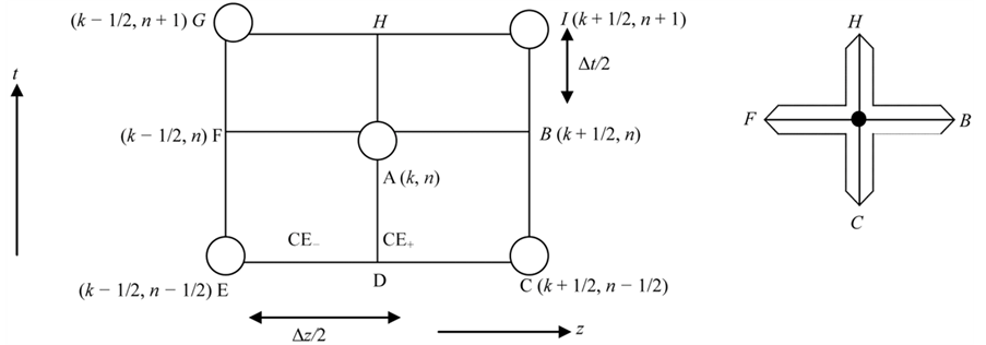
and . j = 0, ±1/2, ±1±3/2, … ±J; k = 0, ±1/2, ±1, ±3/2, … ±K, and n = 0, 1/2, 1, 3/2, … N. At y = 0, j = 0 so we have the corresponding computational stencil for mesh point ·(0, k, n), as shown in Figure 3.
In Figure 3(a), the rhombus ABCD and ADEF constitute a pair of Conservation Elements namely CE+ and CE− respectively. The common/adjoining boundaries of these conservation elements for the mesh point ·(0, k, n) define their solution element as in Figure 3(b). Furthermore, the mesh points are staggered so that the difference between the values of k and n at adjacent nodes alternates between whole numbers and half integers.
3.2. Derivation of the One-Dimensional Advection-Dispersion Scheme
Flux conservation demands that the total flux across a conservation element e.g. ABCD (CE+) and AFED (CE−) in Figure 3(a) should satisfy Equation (12). Consequently, we compute the flux of the contaminant across the boundaries of the conservation elements. To proceedwe define  and
and  as the numerical analogues of
  and
and  on any arbitrary space time node (0, k, n) within the computational region in the neighborhood of Solution Element SE (k, n). The flux across the boundaries of the elements is evaluated as follows;
Flux leaving CE+ through 
On line ; using a first order Taylor series approximation
 (14)
(14)
There is no temporal change on , so that
 .
.
As a result,
 (15a)
(15a)
In this regard,
 (15b)
(15b)
Using this procedure, the total flux across the boundaries of CE+ is given as;
 (16)
(16)
Therefore, the condition for flux balance on this conservation element is given in Equation (17) below.
 (a) (b)
Figure 3. Computational stencil for 1-dimensional CE/SE scheme. (a) Conservation element; (b) Solution element.
Normalizing Equation (17) with , and replacing the groups
 ,
,  and
and  with the Courant number
 ![]() Diffusion number
Diffusion number ![]() and normalized flux
and normalized flux  respectively, we obtain;
 (18a)
(18a)
The complementary part of Equation (18a) is obtained by enforcing flux conservation criterion on the contaminant across the boundaries of CE−. This evaluates to
 (18b)
(18b)
Thus the solution;
 (19a)
(19a)
where
 (19b)
(19b)
 (19c)
(19c)
 (19d)
(19d)
 (19e)
(19e)
 (19f)
(19f)
 (19g)
(19g)
Equation (18) is a one-dimensional CE/SE advectiondispersion (ad) scheme. a is the advection speed and is the coefficient of dispersion. In view of Equation (5), a = 1. Special cases of the ad scheme are the pure advection
 , and the pure dispersion a = 0 schemes. Using the analysis of [13], the a-d scheme is numerically stable provided
  ≤ 1. However, the pure dispersion scheme is unconditionally stable.
3.3. Construction of CE/SE Solution for Dispersion Reaction Transport
To build a CE/SE solution for the reaction dispersion equation in the matrix, and to streamline development, we recall Equation (6) and introduce an arbitrary advection term with speed![]() , thus we have
, thus we have
 (20)
(20)
Using the transformation , Equation (20) becomes
 (21a)
(21a)
In Equation (21a)
 (21b)
(21b)
In view of Equations (19) and (21), Equation (6) has the CE/SE solution
 (22a)
(22a)
Setting  in Equation (20) to obtain the dispersion reaction transport, we have
 (22b)
(22b)
with
 (22c)
(22c)
3.4. Construction of CE/SE Solution for Fracture and Matrix Flow
 is the numerical analogue of the two dimensional distribution of the contaminant in the fracture. The numerical equivalence of Equation (11) for the fracture flow can be represented as;
 (23)
(23)
where
 (24)
(24)
and
 (25)
(25)
Similarly the concentration distribution across the fracture-matrix interface is given as;
 (26)
(26)
and the concentration distribution in the matrix satisfies
 (27)
(27)
where
 (28a)
(28a)
and
 (28b)
(28b)
with
 (28c)
(28c)
Here, we have chosen  the step size across the fracture-matrix interface as
  to stretch computation in the region. Following the results of [17], Equations (20) and (23) lead to numerical schemes of second order accuracy, given that the numerical operators
 ,
,  and
and  are second order in accuracy.
4. Validation of CE/SE Numerical Scheme
To perform an indirect check on the accuracy and validity of CE/SE algorithms developed in Section 3, we consider as a test case the problem of the transient distribution of charge carriers q(x, t) on the normalized base length of an electrical transistor satisfying the following transport model;
 (29a)
(29a)
with
 (29b)
(29b)
 (29c)
(29c)
Here ![]() and k are material constants. They are the drift velocity and the diffusion coefficient of charge carriers along the cross section of the semi-conductor. Equation (29) (a, b and c) has a simple closed form analytical solution given in Equation (30) below.
and k are material constants. They are the drift velocity and the diffusion coefficient of charge carriers along the cross section of the semi-conductor. Equation (29) (a, b and c) has a simple closed form analytical solution given in Equation (30) below.
Comparative performance of the CE/SE scheme relative to the exact solution and the quickest five point’s finite difference scheme are shown on Figures 4 and 5. The chosen values of a, k, Dx, and Dt are identical to the parameters employed for simulations in this work.
In Figure 4, there is a very good agreement between CE/SE and Finite Difference approximations with analytical solution. In this case, absolute errors are evaluated as 0.16% and 0.14% respectively. The corresponding Courant and diffusion numbers for the simulation are 2.56 ´ 10−4 and 7.50 ´ 10−3 respectively. However, in Figure 5, it is seen that the quickest five point finite difference scheme presented in [18] is marginally stable in this regime. The notation b ´ 10±n implies b e ± n.
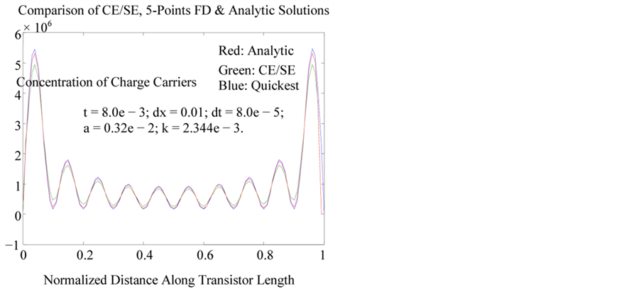
Figure 4. Comparison of CE/SE and finite difference approximations.
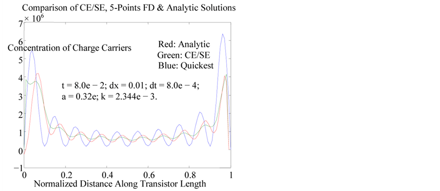
Figure 5. Comparison of CE/SE and finite difference approximations.
5. Discussion of Results
Numerical simulations of fracture/porous matrix flow conditions are performed over an average of 20,000 static conservation elements. Except for redefining the computational step size to stretch the fracture matrix interface, no other mesh refinement algorithm is implemented throughout the physical domain. Our simulation results are the time dependent concentration profiles of contaminant in the fracture and matrix. Simultaneously, we also obtain the time dependent flux variation of the contaminant. This flux variation result is new and it explains some phenomena identified in literature. The CE/SE schemes described in this work are explicit solvers, hence it requires minimal computational resources. This is because it does not require global matrix assembling and inversion processes.
5.1. Response of Profiles in Fracture to Cyclic Loading (Homogeneous Aquifer)
Figures 6 and 7 show the concentration profile of the contaminant in silty clay and fissured limestone aquifers. These distributions are due to one, two and three cycles of fertilizer applications per annum for a period of 30 years.
As shown in Table 1, for these aquifers, we have used identical values of conductivities but different coefficients of dispersion. In line with expectation, concentration profiles in the fracture increase with the frequency of loading. On both figures, the difference between loading two and three cycles per annum is less pronounced than the difference between loading at the rate one and two cycles per annum. Thus, we infer that aquifer response to high frequency of loading is similar to the asymptotic effect of constant loading. Also, these figures show
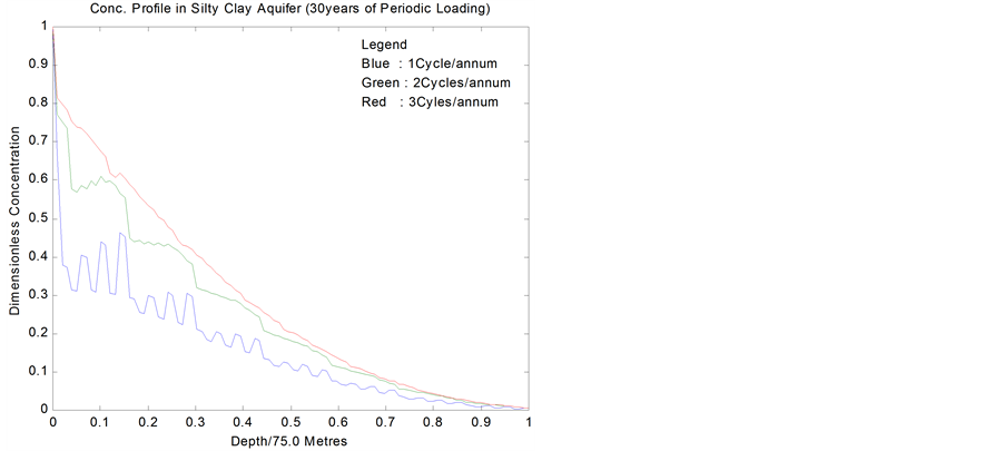
Figure 6. Conc. profiles in silty clay.
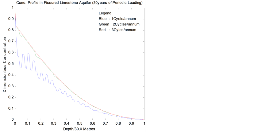
Figure 7. Conc. profiles in fissured limestone.
that the sensitivity of the aquifers to periodic loading is more of a direct function of their dispersivity. Conversely, it can be deduced that the dispersion coefficient of a contaminant in an aquifer depends on its loading history. These figures further show that an increase in the dispersion coefficients in the fracture will accelerate solute arrival time.
Theoretical basis for the wavy patterns of the concentration profiles is provided in [19]. In addition, these profiles correctly simulate the patterns of field observations of nitrate profile under agricultural land published in [20]. This is the first work that recovers the field profile of nitrate under agricultural soil.
However, Figure 8 shows that for consolidated formations with mean conductivity less than 10−6, cyclic loading has a negligible effect on the contaminant profile. On

Table 1 . Typical hydrological parameters of some sedimentary formations.
Adapted from [22].
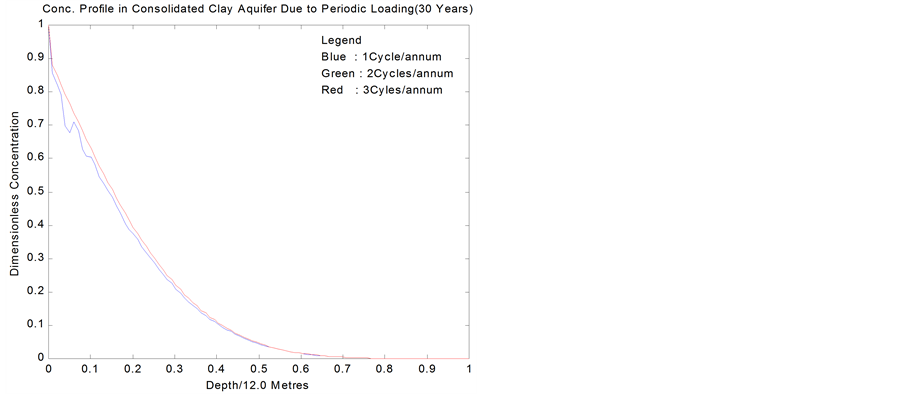
Figure 8. Conc. profile in consolidated clay after 30 yrs.
the other hand, when compared with Figure 7; Figure 9 illustrates the effect of loading duration on contaminant font in a relatively permeable fissured limestone aquifer. Sustained periodic loading rectifies the wavy pattern of nitrate profile and marginally increase its breakthrough depth.
5.2. Corresponding Response of the Matrix
Figure 10 shows representative concentration distribution at various depths in the matrix block separating two fractures in a typical loose clay aquifer loaded at two cycles per annum for thirty years.
Similarly, Figure 11 shows the corresponding concentration distribution at various depths in the matrix of limestone formation loaded at the same frequency over a period of hundred years.
The profiles in the matrix indicate storage in regions adjacent to the fracture. This delays the progress of the
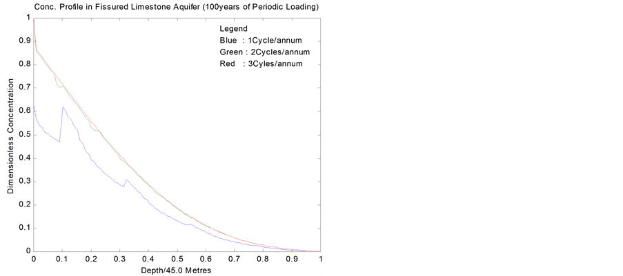
Figure 9. Conc. profile in fissured limestone after 100 yrs.
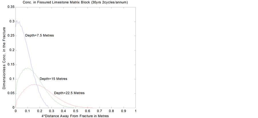
Figure 10. Profile in fissured limestone matrix.
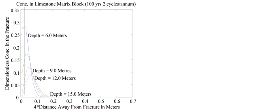
Figure 11. Profile in limestone matrix.
contaminant in the fracture. As shown on Figures 10 and 11, the storing process continues until the matrix saturation limit at the depth is attained. Beyond this saturated zone, the contaminant proceeds through a non-linear diffusion process. Consequently, solute concentration in layers adjacent to the fracture in the matrix at certain depths in the aquifer tends to be slightly higher than the concentration in the fracture, especially in formations with very low conductivity.
In addition to the breakthrough curves, CE/SE now facilitates a more illuminating analysis of the effect of matrix diffusion through an investigation of the pattern of solute flux across the fracture/matrix interface. The flux corresponding to the profiles in Figures 10 and 11 are shown in Figures 12 and 13 respectively. Close to the wall of the fracture, the flux of the solute changes from positive values to negative values as we go down the
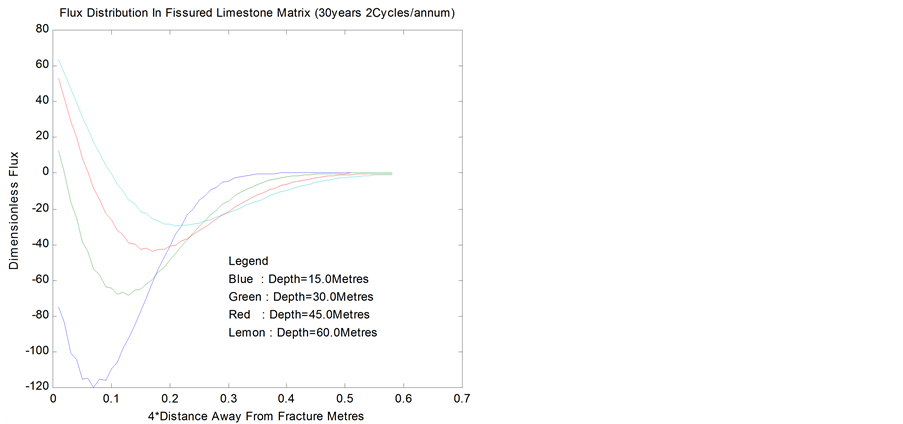
Figure 12. Flux dist profile in fissured limestone matrix.
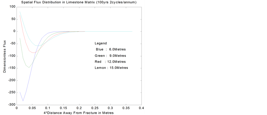
Figure 13. Flux dist profile in limestone matrix.
depth of the aquifer. This suggests that the matrix has the tendency to feed the fracture at certain locations where advective transport is slower than diffusive transport or when flow in the fracture is off season.
Thus, Figures 12 and 13 explain the observation made by [21] associated with the difficulty of finite element method to evaluate contaminant flux at the interface between fracture and matrix. Equally important remark is that the solute flux vanished with distance into the matrix. This behavior satisfies the no flux condition specified on the matrix centerline y = x by [13]. This condition is also prescribed in our complementary boundary condition Equation (7d). These profiles further validate the consistency and efficacy of the CE/SE in this regime.
5.3. Effects of Stratification
Figure 14 represents the response of a 50% Loose/50% Consolidated Clay system to 1, 2 and 3 cycles/annum loadings over 50 years duration. The behavior of the upper stratum is identical to what obtains in homogeneous loose clay aquifer; shown in Figure 6. However, the lower consolidated formation acts to protect aquifers deeper than 37.5 meters from contamination. Loading frequency does not affect the amount of solute crossing the interface. Rather, the contaminant builds up in the upper stratum. This effect is well pronounced in Figure 14, which shows the time response for Loose Clay/Consolidated Clay stratified system.
The presence of an accumulation zone at the interface between the two strata is evident. This effect is pronounced when the ratio of the conductivities or dispersion coefficients of the upper to the lower formation is of the order of 10p with p ³ 1.0.
Another important feature of the breakthrough curves in Figures 14 and 15 is the relative degree of refraction
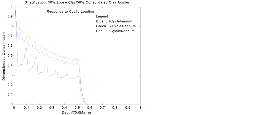
Figure 14. Effect of loading frequency duration loading in stratified aquifer.
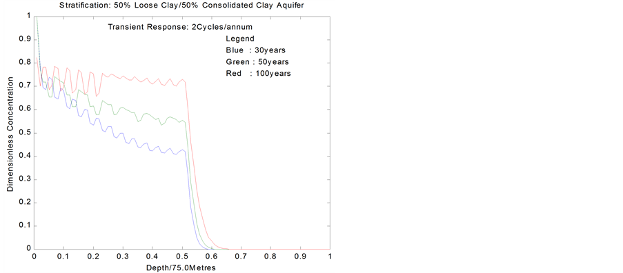
Figure 15. Effect of loading in stratified aquifer.
of the profiles at the interface between two strata. Clearly, the CE/SE method has an exceptional ability to handle stratification. The angle of refraction depends on the relative conductivity and dispersion coefficient of the neighboring strata. Also, mild variation in either the conductivity or dispersion coefficient of a geological system is sufficient to modulate stratification.
On the other hand, Figure 16 illustrates the effects of the geological log on the breakthrough curves of contaminant in a stratified aquifer. The loading frequency for this study is two cycles per annum for duration of 50 years. In the 20A/80B composition, the upper stratum is heavily polluted. Consequently, water wells that are less than 20 meters in depth in such an aquifer are unsafe for domestic consumption even when the concentration of nitrate on topsoil is just 10.0 ppm. Also, if the solute concentration on topsoil is greater than 18.0 ppm, wells that are less than 37.5 m in depths will be unsafe for drinking using WHO standards of maximum of 10 ppm of nitrate in drinking water.
Similarly, in the 80A/20B composition the minimum depth to safe water is 60.0 meters if nitrate concentrations in excess of 50.0 ppm on topsoil. Clearly, the composition of a stratified aquifer determines its susceptibility to pollution. Next, we look at the effects of ordering of layers on relative susceptibility of stratified aquifers. The breakthrough curves corresponding to 80A/20B and 20B/80A arrangement of layers in a binary system are shown in Figure 17. While depth to safe water lies below 60.0 meters for nitrate concentration in excess of 50.0 ppm on topsoil in the 80A/20B system, wells in the 20B/80A arrangement are safe for drinking so long as their bottom is deeper than 10.0 meters into the aquifer. Evidently, contaminant profile in multi-layered systems largely depends on the ordering of the layers.
Figure 17 is the outcome of numerical exercise to re-
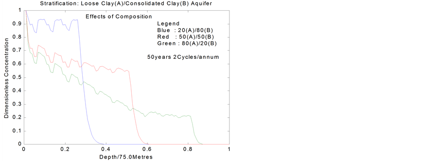
Figure 16. Effects of stratification of aquifer on profile of breakthrough curve.
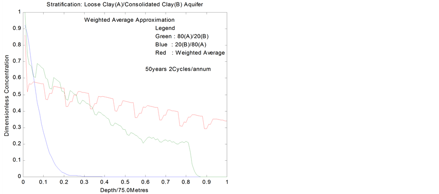
Figure 17. Effects of parameters averaging profile of breakthrough curve.
place the 80A/20B and the 20B/80A systems with an equivalent aquifer whose hydraulic parameters are the weighted averages and mean hydrological parameters of constituents. Clearly, this approach is misleading due to sharp variations in properties. Similar results are obtained even when the conductivities are comparable but with significant difference in coefficients of dispersion.
Similarly, Figure 18 describes the concentration distribution in cretaceous clay (u = 9.6e − 5 m/day, D = 5.43e − 3 m2/day) underlain with fissured limestone. The figure shows that mean value or weighted average approach to system’s simplification in stratified aquifers can be used to optimize computational cost provided the conductivities and dispersion coefficients of adjacent layers are relatively close.
6. Conclusion
In recognition of the importance of protecting freshwater
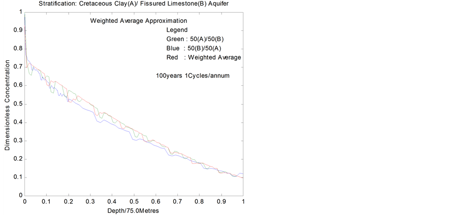
Figure 18. Effects of parameters averaging in formations with converging properties.
aquifers from aqueous phase liquid contaminants, this work presents the development and application of an advection-dispersion-reaction a-d-r Space-Time Conservation Element/Solution Element (CE/SE) numerical scheme for contaminant tracking in fractured porous media. Using flux splitting approach, a two-dimensional CE/SE scheme is developed for simulating the evolution and fate of aqueous phase liquid contaminant in stratified fractured porous media. Thus, the CE/SE scheme is herein extended to handle geological time scale problems. The developed scheme is able to resolve some of the issues associated with numerical solution of groundwater contaminant hydrology problems. Such difficulties include the use of ideal initial/boundary conditions and parametric jumps that may be due to stratification or scale effects. To simulate the Nigerian experience of nitrate pollution of freshwater aquifers; we have deployed the developed scheme to solve the advection-dispersionreaction a-d-r equation in geologic media under a time periodic Dirichelet type boundary condition. This models the actual pattern of aqueous phase contaminant on arable agricultural lands. It is established that the CE/SE method is a viable and efficient tool for tracking contaminant transport in geologic profiles. The scheme is able to sense order of 10−3 variation in hydrological properties of aquifers. It is also shown that attempts at systems simplification in heterogeneous reservoirs through the use of mean or weighted average values of hydrological parameters are in error unless the hydro-geological properties of neighboring geological formations are very close. The developed model was validated with analytical and the quickest five points finite difference scheme. CE/SE is computationally inexpensive and easily programmed.
REFERENCES
- X. Wang, S. Chang and P. C. Jorgenson, “Accuracy Study of Space-Time CE/SE Methods for Computational Aero-Acoustic Problems involving Shock Waves,” Proceedings of the 38th Aerospace Sciences Meeting & Exhibition, Reno, 10-13 January 2000, AIAA2000-0865.
- Y. Chen and L. J. Durlofsky, “An Adaptive Local-Global up Scaling for General Flow Scenario in Heterogeneous Formations,” Transport in Porous Media, Vol. 62, No. 2, 2006, pp. 157-185. http://dx.doi.org/10.1007/s11242-005-0619-7
- A. El-Zein, J. P. Carter and W. Airey, “Three-Dimensional Finite Elements for the Analysis of Soil Contamination Using a Multiple-Porosity Approach,” International Journal for Numerical and Analytical Methods in Geomechanics, Vol. 30, No. 7, 2006, pp. 577-597. http://dx.doi.org/10.1002/nag.491
- R. J. LeVeque, “Numerical Methods for Conservation Laws, Lecture in Mathematics Series,” Birkhauser Verlag, Basel, 1992. http://dx.doi.org/10.1007/978-3-0348-8629-1
- D. De Cogan and A. De Cogan, “Applied Numerical Modeling for Engineers,” Oxford University Press, New York, 1997.
- J. F. Botha and J. P. Verwey, “Aquifer Test Data and Numerical Models,” In: T. F. Russell, Ed., Computational Methods in Water Resources IX, Elsevier, New York, 1992, pp. 459-466.
- S. A. Sadrnejad, A. Ghasemzadeh, A. S. Ghoreishian and G. H. Montazeri, “A Control Volume Based Finite Element Method for Simulating Incompressible Two-Phase Flow in Heterogeneous Porous Media and Its Application to Reservoir Engineering,” Petroleum Science, Vol. 9, No. 4, 2012, pp. 485-497. http://dx.doi.org/10.1007/s12182-012-0233-6
- A. El-Zein, J. Carter and D. Airey, “Multiple-Porosity Contaminant Transport by Finite-Element Method,” International Journal of Geomechanics, Vol. 5, No. 1, 2005, pp. 24-34.
- I. Herera, “Localized Adjoint Method: Topics for Further Research and Some Contributions,” In: T. F. Russell, Ed., Computational Methods in Water Resources IX, Elsevier, New York, 1992, pp. 3-17.
- G. Matheron and G. De Marsily, “Is Transport in Porous Media Always Diffusive? A Counter Example,” Water Resources Research, Vol. 16, No. 5, 1980, pp. 901-917. http://dx.doi.org/10.1029/WR016i005p00901
- M. Xiang and Z. Nicholas, “A Stochastic Mixed Finite Element Heterogeneous Multi-Scale Method for Flow in Porous Media,” Journal of Computational Physics, Vol. 230, No. 12, 2011, pp. 4696-4722. http://dx.doi.org/10.1016/j.jcp.2011.03.001
- M. Ibaraki and E. A. Sudiky, “Colloids-Facilitated Contaminant Transport in Discretely Fractured Porous Media, 1. Numerical Formulation and Sensitivity Analysis,” Water Resources Research, Vol. 31, No. 12, 1995, pp. 2945- 2960. http://dx.doi.org/10.1029/95WR02180
- S. C. Chang, “The Method of Space-Time Conservation Element and Solution Element, a New Approach for Solving the Navier-Stokes and Euler Equations,” Journal of Computational Physics, Vol. 119, No. 2, 1995, pp. 295-324. http://dx.doi.org/10.1006/jcph.1995.1137
- S. C. Chang, X. Wang and C. Chow, “The Space-Time Conservation Element and Solution Element Method: A New High Resolution and Genuinely Multidimensional Paradigm for Solving Conservation Laws,” Journal of Computational Physics, Vol. 156, No. 1, 1999, pp. 89- 136. http://dx.doi.org/10.1006/jcph.1999.6354
- E. A. Sudiky and E. O. Frind, “Contaminant Transport in Fractured Porous Media: Analytical Solution for a System of Parallel Fractures,” Water Resources Research, Vol. 18, No. 6, 1982, pp. 1634-1642. http://dx.doi.org/10.1029/WR018i006p01634
- K. Hutter and V. O. S. Olunloyo, “On the Distribution of Stress and Velocity in an Ice Strip, Which Is Partly Sliding over and Partly Adhering to Its Bed, by Using a Newtonian Viscous Approximation,” Proceeding Royal Society London, Vol. 373, No. 1754, 1980, pp. 385-403. http://dx.doi.org/10.1098/rspa.1980.0155
- R. J. LeVeque, “A Well-Balanced Path-Integral f-Wave Method for Hyperbolic Problems with Source Terms,” Journal of Scientific Computing, Vol. 48, No. 1-3, 2011, pp. 209-226. http://dx.doi.org/10.1007/s10915-010-9411-0
- L. Leonard, “Simple High-Accuracy Resolution Program for Convective Modeling of Discontinuities,” International Journal of Numerical Methods in Fluids, Vol. 8, No. 10, 1988, pp. 1291-1318. http://dx.doi.org/10.1002/fld.1650081013
- P. Grindrod, “The Theory and Applications of Reaction Diffusion Equations: Patterns and Waves,” Oxford Applied Mathematics and Computing Series, Clarendon Press, Oxford, 1996.
- S. Mallick and S. Banerji, “Nitrate Pollution of Groundwater as a Result of Agricultural Development in Indogangan Plain, India,” Quality of Groundwater; Proceedings of International Symposium Noordwijkerhunt, Netherlands, 23-28 March 1981, pp. 17-38.
- J. Noorisand and M. Mehran, “An Upstream Finite Element Method for Solution of Transient Transport Equation in Porous Media,” Water Resources Research, Vol. 18, No. 3, 1982, pp. 588-596. http://dx.doi.org/10.1029/WR018i003p00588
- V. O. S. Olunloyo, O. Ibidapo-Obe and T. A. Fashanu, “An Image Processing Approach for the Characterization of Hazardous Agricultural Waste Transport in Multilayered Soils and Aquifers,” Proceedings 4th World Congress of Computers in Agriculture and Natural Resources, Orlando, 24-26 July 2006, pp. 717-726.