Open Journal of Fluid Dynamics
Vol.06 No.04(2016), Article ID:71396,7 pages
10.4236/ojfd.2016.64021
A Theoretical Solution for the Reynolds Stress: Validations in Canonical Flow Geometries
Taewoo Lee
Mechanical and Aerospace Engineering, SEMTE Arizona State University, Tempe, USA

Copyright © 2016 by author and Scientific Research Publishing Inc.
This work is licensed under the Creative Commons Attribution International License (CC BY 4.0).
http://creativecommons.org/licenses/by/4.0/


Received: September 19, 2016; Accepted: October 18, 2016; Published: October 21, 2016
ABSTRACT
A theoretical approach is developed for solving for the Reynolds stress in turbulent flows, and is validated for canonical flow geometries (flow over a flat plate, rectangular channel flow, and free turbulent jet). The theory is based on the turbulence momentum equation cast in a coordinate frame moving with the mean flow. The formulation leads to an ordinary differential equation for the Reynolds stress, which can either be integrated to provide parameterization in terms of turbulence parameters or can be solved numerically for closure in simple geometries. Results thus far indicate that the good agreement between the current theoretical and experimental/DNS (direct numerical simulation) data is not a fortuitous coincidence, and in the least it works quite well in sensible ways in canonical flow geometries. A closed-form solution for the Reynolds stress is found in terms of the root variables, such as the mean velocity, velocity gradient, turbulence kinetic energy and a viscous term. The form of the solution also provides radically new insight on how the Reynolds stress is generated and distributed.
Keywords:
Turbulence Theory

1. Introduction
We present a theoretical development and a solution for the Reynolds stress in turbulence. Turbulence is considered one of the most difficult problems in fluid physics, or some say, physics in general. It is also quite important as many issues of practical concern, such as weather, aerodynamics, combustion flows and many industrial processes depend on turbulence, and much work has been done on finding some adequate approximations so that immediate problems of turbulent flows can be solved (we do not attempt to list the vast literature in this area). As finding the entire absolute (mean + fluctuations) velocity field is quite difficult, or as some argue an overflow of information, here we focus on finding the Reynolds stress as a function of the “root” turbulence parameters, such as the mean velocity and its gradient, turbulence kinetic energy, in particular its longitudinal component, and also a viscous term. This has been the goal of turbulence theory and modeling: parameterizing the Reynolds stress in terms of known or readily available variables, or so-called the closure problem.
2. Mathematical Formulation
The current theoretical framework leads to the “integral formula” explicitly giving the Reynolds stress in terms of the “root”, calculatable turbulence parameters. In Reynolds-averaged Navier-Stokes (RANS) equation, non-linear terms involving turbulent fluctuation velocities arise since the absolute velocity is decomposed into mean (U) and fluctuating ( ) component:
 . The non-linear terms that develop during the averaging process in the RANS are called the Reynolds stress, which involves time-averaged components of products of fluctuating velocities,
 . Here, we omit the bar above
 , etc., for simplicity, and take the fluctuation parameters to be time-averaged. Figuring out how the Reynolds stress is related to the mean and other “root” turbulent parameters has been the topic of numerous studies, for quite some time. However, we notice that the decomposition is necessary only in the absolute coordinate frame, and if we move or displace the control volume at the mean speed of the flow (see Figure 1) then the mean velocity drops out of the momentum equation. That is, RANS is greatly simplified in the relative coordinate frame, or for a control volume moving at the mean velocity of the fluid. Therefore, the x-momentum equation, for an incompressible boundary-layer flow, becomes:
 (1)
(1)
In Equation (1), t, x, and y are the time and coordinates, while ,
,  , and
, and  are the turbulent fluctuations with respect to the mean.
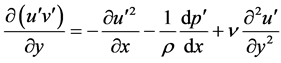
If the time mean of the fluctuating velocity does not vary appreciably in time, then we can write a “steady-state” momentum equation, and solve for the gradient of the Reynolds stress.

Figure 1. A schematic illustration of the concept of the theory.
 (2)
(2)
In conventional calculations, the x-derivatives would have been set to zero for fully-developed flows, and we would be left with a triviality. However, we note that Equations (1) and (2) have been written for a control volume which is moving along with the mean flow velocity, as shown in Figure 1 for a boundary-layer flow as an example. For a flow over a flat plate, the boundary layer grows due to the “displacement” effect. The mass is displaced due to the fluid slowing down at the wall, as is the momentum, and it turns out other turbulence parameters as well. The boundary layer thickness grows at a predictable rate, depending on the Reynolds number. Thus, if one rides with the fluid moving at the mean velocity, one would see a change in the all of the turbulence properties, as illustrated in Figure 1. This displacement effect can be mathematically expressed as:
 (3)
(3)
The mean velocity, U, appears as a multiplicative factor in Equation (3). C1 is a constant that depends on the Reynolds number. Similarly, the gradient of the pressure fluctuation will not be zero in general. However, this term is expected to be significant only for compressible flows, so we omit this term from further analysis in this phase of the work. In Equation (2), we now have a simple integrable expression to find the Reynolds stress, after using Equation (3). If we integrate by parts, we obtain:
 (4)
(4)
For axi-symmetric flow, the results are similar, leading to the following expression for the Reynolds stress.
 (5)
(5)
3. Results and Discussion
Figure 2 shows the comparison of the Reynolds stress obtained from Equation (4) with experimental data of DeGraaf and Eaton [1] . In that work, data on various turbulence quantities and the Reynolds stress (all normalized by the friction velocity) are provided, and also various scaling approaches tested with the data, in a well-designed experiment for flows over a flat plate with zero pressure gradient. The Reynolds number based on the momentum thickness (Reθ) ranged from 1430 to 31,000 [1] . In Equation (2), we use their measured parameters, U and , and input them into Equation (4). Gradients of U and
  are calculated from the experimental data. As the experimental data are discontinuous, and at times hard to transcribe, there are some fluctuations and potential errors in the final calculations of the Reynolds stress, particularly close to the wall where the gradients are very steep and the data points all clustered. We can nonetheless input the root parameters into Equation (4) to compute accordingly, and compare with

Figure 2. Comparison of the Reynolds stress in boundary layer flows over a flat plate. The data (symbols) are for Reθ = 1430 - 31,000 [1] . Lines represent current result (Equation (4)), which are identified the color from pink (triangle data symbol) for Reθ = 1430 to blue (circle data symbol) to Reθ 31,000.
the measured Reynolds stress as in Figure 2. In spite of dealing with discontinuous experimental data and their gradients, the comparison of Equation (4) result with experimentally observed Reynolds stress is in general quite good.
 profiles have a sharp negative peak, near the wall, and gradually decrease as the distance from the wall increases [1] [2] . Although this is somewhat attenuated by the mean velocity term in Equation (1) (the first term on the RHS of Equation (4)), the resulting contribution of
  is still high near the wall. However, the sharp peaks in the
  are also associated with a large gradient in
 , which increases the magnitude of the viscous “dissipation” term, offsetting the large “transport” effect. As noted above, dealing with experimental data does lead to some errors, and some “leakage” in the Reynolds stress is found in Figure 2. Unless the gradients are accurately entered as input, and their y coordinates are perfectly aligned, this kind of leakage can occur. Also, the method is not able to track the Reynolds stress at the lowest Reynolds number close to the wall for the same reason, which is somewhat surprising as the requirements for spatial and measurement resolutions are the least at that condition.
Figure 3 is a similar comparison of Reynolds stress as calculated by Equation (4), with DNS results for fully-developed channel flows [3] [4] . DNS results are highly resolved (we had access to the entire data set through the authors’ website [4] ), and continuous, and therefore inputting the root parameters and taking the gradients do not lead to much fluctuations or misalignments, as was the case in Figure 2. Iwamoto and co-workers [3] [4] have performed DNS, using established methods [3] [4] for Reτ = 110 - 650, where Reτ is the Reynolds number based on the friction velocity and channel half-width. The entire data set from the DNS is available on their website [4] , including

Figure 3. Comparison of the Reynolds stress in boundary layer flows over a flat plate. Lines are theoretical results, using Equation (4). Data symbols: circle (Reτ = 110), diamond (150), square (300), triangle (400), + (650). Line that track the data correspond to the same Reynolds number.
the mean velocity, turbulent fluctuating velocity components, and various moments of their products. We input the necessary root turbulence parameters into Equation (4), and compare with the Reynolds stress from DNS. The agreement is nearly perfect at low Reynolds numbers in Figure 3, which gives some confidence that we have captured the true physics of turbulent transport, and that the results are not a fortuitous coincidence.
There is an interesting departure at higher Reynolds numbers, as the solution starts to overshoot the DNS data as y approaches the centerline. The y location where this departure starts to occur decreases (further away from the centerline) at higher Reynolds numbers. This departure is due to the fact that the symmetry boundary condition for channel flows, at the centerline, has not yet been imposed. As noted earlier, the integral term is a “displacement” term accumulating from the wall, and at the centerline the displacement must cancel out. For example, the integral formula (Equation (4)) and its preceding transport equation (Equation (3)) have been derived for flows bounded on one side, such as the flow over a flat plate, and the solution proceeds from y = 0 (wall) onward. For channel flows, the flow is bounded on both sides, leading to the requisite symmetry condition at the centerline. One way to impose the symmetry boundary condition is to force the constant C1 to be proportional to the velocity gradient. For example,
 (6)
(6)
With m = 1/3, indeed the calculated Reynolds stress tracks the DNS data fairly well at the Reynolds number of 400, as shown in Figure 4. There are small undulations now that derivatives of mean flow velocity are used in the multiplicative constant. Although this approach may not seem so elegant, Equations (3) and (4) have been derived based on the displacement of turbulence parameters, so that symmetry or other boundary conditions should be applied as in Equation (6). For low Reynolds numbers, the displacement apparently is insignificant and Equation (6) was not needed, as shown in Figure 3.
4. Conclusions
We have found a method to derive an expression for the Reynolds stress in simple flow geometries, leading to an “integral formula”. This formula, and the method, works quite well in determining the Reynolds stress based on inputs of root turbulence parameters, such as streamwise component of the turbulence kinetic energy, the mean velocity and its gradient. The predicted Reynolds stress is in good agreement with experimental and DNS data. In particular, if the data are continuous and aligned, then agreement is nearly perfect. There are some nuances and corrections that need to be examined, such as applying symmetry boundary conditions and relating the displacement effect to the flow geometry and Reynolds number. Thus far, the theory has been tested against relatively simple geometries. Would this method be useful in full three- dimensional turbulent flows? That is a question that is being thought of at this time. The fact that u'v' is related to u'2 is easier to implement in computational applications as the turbulent kinetic energy can be related to u'2, assuming isotropy, or an equation for u'2 can be numerically solved in conjunction with Equation (4). For simple flows, the displacement effect could be effectively treated with Equation (6). Extensions to fully three-dimensional flows will require this displacement effect to be parameterized,

Figure 4. Correction for the symmetry condition, using Equation (6). Reτ = 400.
which may not be a simple matter. On the other hand, it was considered difficult to parameterize the Reynolds stress even in simple flows, for quite some time.
Acknowledgements
This work was conceived immediately after some conversations with friend (s) in Brno, Czech Republic, on Cesky Drahy train which allows for the window to be opened at turbulent relative airspeeds.
Cite this paper
Lee, T. (2016) A Theoretical Solution for the Reynolds Stress: Validations in Canonical Flow Geometries. Open Journal of Fluid Dynamics, 6, 272- 278. http://dx.doi.org/10.4236/ojfd.2016.64021
References
- 1. DeGraaf, D.B. and Eaton, J.K. (2000) Reynolds Number Scaling of the Flat-Plate Turbulent Boundary Layer. Journal of Fluid Mechanics, 422, 319-346. http://dx.doi.org/10.1017/S0022112000001713
- 2. Hinze, J.O. (1959) Turbulence. 2nd Edition, McGraw Hill, New York.
- 3. Iwamoto, K., Sasaki, Y. and Nobuhide K. (2002) Reynolds Number Effects on Wall Turbulence: Toward Effective Feedback Control. International Journal of Heat and Fluid Flows, 23, 678-689.
http://dx.doi.org/10.1016/S0142-727X(02)00164-9 - 4. Iwamoto, K. and Kasagi, N. List of DNS Databases (as of Sepember 16, 2004).
http://thtlab.jp/DNS/dns_database.html