Open Journal of Fluid Dynamics
Vol.2 No.3(2012), Article ID:22536,9 pages DOI:10.4236/ojfd.2012.23006
CFD Simulations for Sensitivity Analysis of Different Parameters to the Wake Characteristics of Tidal Turbine
Department College of Engineering, Mathematic and Physical Sciences, University of Exeter, Exeter, UK
Email: mgg204@exeter.ac.uk
Received June 26, 2012; revised July 30, 2012; accepted August 16, 2012
Keywords: IBF Model; LES; MRL Turbine; Grid Size; Width Proximity
ABSTRACT
This paper investigates the sensitivity of width proximity and mesh grid size to the wake characteristics of Momentum Reversal Lift (MRL) turbine using a new computational fluid dynamics (CFD) based Immersed Body Force (IBF) model. This model has been added as a source term into the large eddy simulation (LES), which is developed for solving two phase fluids. The open source CFD code OpenFOAM was used for the simulations. The simulation results showed that the grid size and width proximity have had massive impact on the flow characteristics and the computational cost of the tidal turbine. A fine grid size and large width inflicted longer computational time. In contrast, a coarse grid size and small width reduced the computational time but showed poor description of the flow features. In addition, a close proximity of the domain’s wall boundary to the turbine affected the free surface, the air body, and the flow characteristics at the interface between the two phases. These results showed that careful investigation of a suitable grid size and spacing between the wall boundary and the turbine are important to minimise the effect of these parameters on the simulation results.
1. Introduction
The interest of exploiting tidal energy using tidal stream devices has been growing rapidly recently. As a result, several studies have been carried out on evaluating the environmental impacts and locating the potential sites as documented by [1-3]. A wide range of tidal stream device designs are currently under development and testing with the aim of improving the efficiency of conventional tidal turbines.
University of Exeter together with Aquascientific Ltd., a small firm located in Exeter, have been working on the development of new design of tidal turbines as part of their research on renewable energies and come up with a novel design called Momentum Reversal Lift, which is currently in the prototype and testing phase. This turbine is a development of cycloidal turbines and as such has a system of three symmetrical blades which revolve through 180˚ for every full rotation of the main shaft. This clearly induces very complex, highly sheared internal flows plus a large circulation flows. Experimental studies have been performed on a small scale MRL models to determine the operating efficiency of the turbine in a fluid test tunnel. However, it is expensive to perform experimental works to study the device parameters in a large scale and or arrays. Therefore, it is crucial to utilize other options such as numerical simulations, which are potentially less expensive.
Numerical models have showed great success in the study of tidal turbines though there are still issues to resolve. Several studies have been carried out using the actuator disc method, such as the simulation of two dimensional flow past a turbine with a free surface by [4], simulation of a horizontal axis turbine and comparison of the far wake with experimental data [5,6], and for the study of close proximity [7]. Studies by [5,7,8] indicate that the above method minimizes the requirement of mesh refinement and of modelling the geometry in full, thus reducing the associated computational costs. The technique has shown good agreement with experimental data but [5] acknowledged that the vortex shedding from the edge of the disc is not similar to the real turbines. The study by [7] also indicates that the actuator disc method has no capability of resolving the flow around each blade except reducing the momentum of the fluid as it passes through the disc.
Detailed modelling of such a system with complex internal motions is a good candidate for overset meshing and/or sliding mesh methods. However, the cost of these methods is high for modelling a large scale or farm scale array tidal turbines, hence a simplified CFD based, Immersed Body Force (IBF) model has been developed for the simulation of the MRL turbine to understand the flow features during energy extraction from the stream flow. The IBF model has been used to investigate the surface deformation, wake recovery and turbine to turbine interactions and other related issues by the same authors [9] and showed better capability of simulating tidal turbines compared to the actuator disc method. This model has been successfully validated with experimental results carried out to calibrate the energy extraction by the MRL turbine, which is currently under-review for publication.
The aim of this paper is therefore to use the IBF model for investigating the effect of width proximity and mesh grid size to the wake characteristics of the MRL turbine. The results will provide the required knowledge on the capability of the IBF model in examining the flow features and other associated parameters and strengthen the confidence to use this model for the study of other turbine technologies, such as wind turbines.
2. Computational Modelling
Complex turbulent motions such as the flows around a tidal turbine can be described by the unsteady Navierstokes equations combined with the continuity equation. Direct Numerical simulation (DNS) has been used to solve the Navier-stokes equations by resolving all the motions and is proved to be the most accurate approach for turbulence simulations [10]. However; DNS needs very fine grid size to effectively resolve the small scale motions making it computationally very expensive.
Therefore, turbulence modelling has been extensively developed to get the balance between the computational cost and the satisfaction of the engineering solutions for the descriptions of turbulent motion. The most popular and often utilized models in the simulation of turbulent motions are Reynolds averaged Navier-stokes (RANS) and large eddy simulation (LES). These models showed success in replacing the DNS.
RANS equations are obtained by statistical averaging of the equations of motion. These averaged equations require the introduction of turbulence models, such as the  model. These turbulence models are used to model all the large and small scale motions and depend on the average flow quantities or modelled approximations. However, all RANS models suffer for the deficiency that they fail to resolve any of the fluctuating scales in the flow. Thus, in cases where the large scale turbulent motions are important, it is necessary to employ the alternative, LES methods. The LES was therefore chosen in this study in order to balance the weakness and strength of the DNS and RANS.
2.1. LES Governing Equations
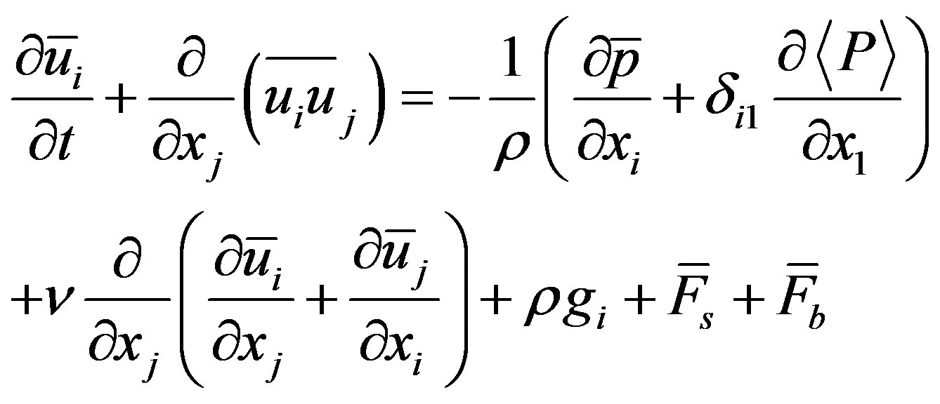
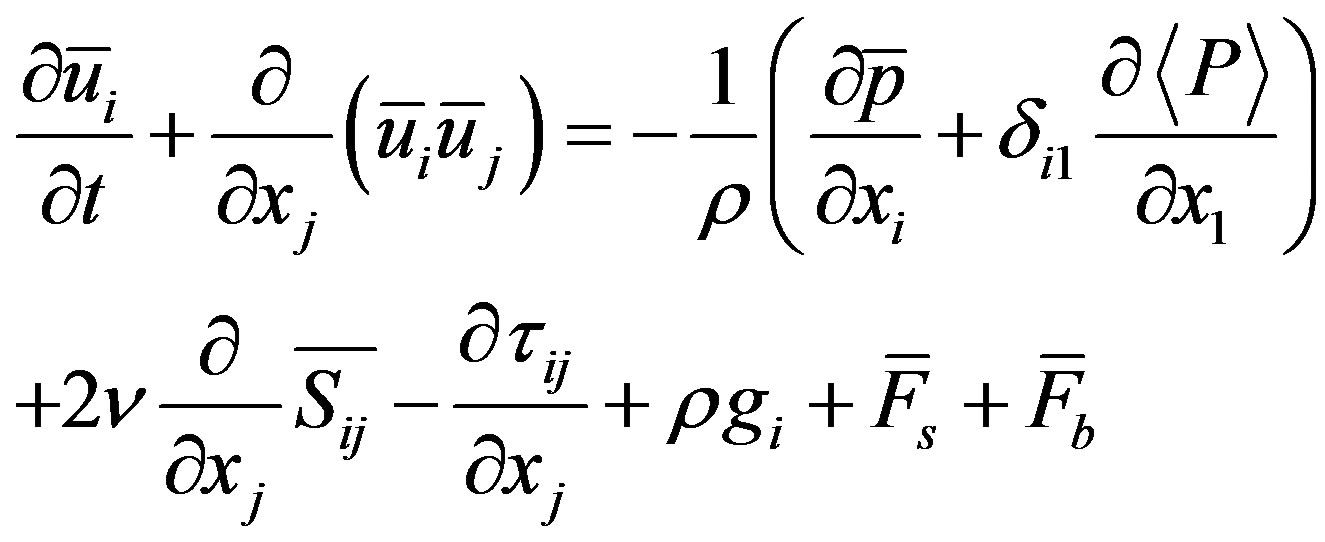
The LES governing equation utilized for the simulation is a combination of the filtered NS equations and source terms as shown in (1). The existing NS equation is developed for solving two incompressible fluids capturing the interface using a VOF method [11]. In this study, a new source term, forcing function , was added to the existing LES model to create a momentum change in the fluid flow by the turbine blades. The filtered NS equations for incompressible flow produce a set of equations [12] that can be defined as:
 (1)
(1)
but the continuity equation does not change by the filtering process because of its linearity and can be written as:
 (2)
(2)
where the bar  is the grid filter operator,
  is the filtered velocity,
  is the filtered pressure, ν is a dimensionless kinematic viscosity,
  is the Kroneckerdelta, and
  is the driving force which vanishes if periodic inlet-outlet boundary conditions are not applied.
Since , the filtered convection term
  is the cause of difficulty in LES modelling because of its non-linearity. Ref. [13] introduced a modelling approximation for the difference of the two inequalities and splits them as:
 (3)
(3)
where the new linking term  is the SGS Reynolds stress. Combining (1) and (3), the filtered NS equations can be rewritten as:
 (4)
(4)
where  is the strain rate of the large scales or resolved scales and is defined as:
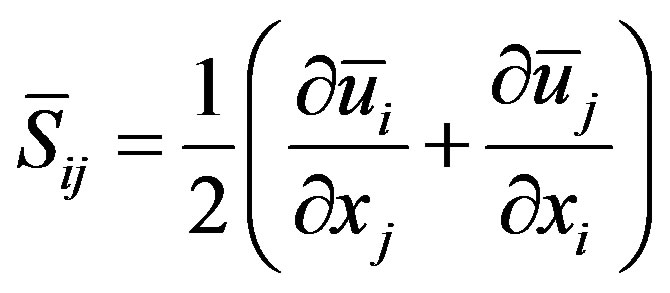 (5)
(5)
The SGS Reynolds stress has to be approximated by using SGS models to get a full solution for the NS equations. The one-equation eddy viscosity SGS model (oneEqEddy) developed by [14] has been used in a wide range of turbulent problems and was used to model the small-scale motions in the MRL turbine simulation. Based on the oneEqEddy model [14], the sub-grid stresses are defined as:
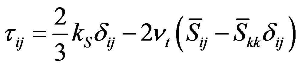 (6)
(6)
where  is the SGS eddy viscosity given as:
 (7)
(7)
and the sub-grid kinetic energy  is given as:
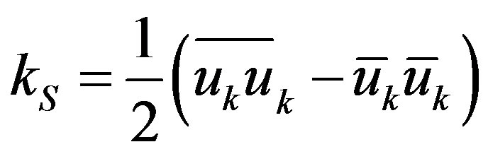 (8)
(8)
where: .
.
2.2. Volume of Fluid Method
The MRL turbine is designed to operate relatively close to the water surface and the dynamics of the free surface will be important for the overall behavior of the turbine. The VOF method has been widely used in the study of floating body applications, breaking waves, non linear free surface flows and other multiphase flows to handle these kinds of problems, as documented by [15-18]. It is an easy, flexible and efficient method for treating free boundaries as described by [19] and was used in this study coupled with the LES model.
The volume of water in a cell is calculated as , where
  is the volume of a computational cell and α is the water fraction of a cell. If the cell is completely filled with fluid then
  and if it is void then its value should be 0. The interface between the phases is represented by values of
  between 0 and 1.
The value of  is calculated from a separate transport equation as:
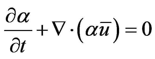 (9)
(9)
During the simulations, there is a surface compression and in OpenFOAM, an extra artificial compression term which is active only on the interface region is introduced into (9) as follows:
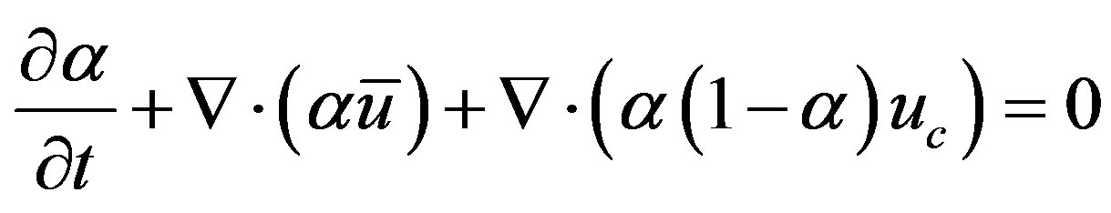 (10)
(10)
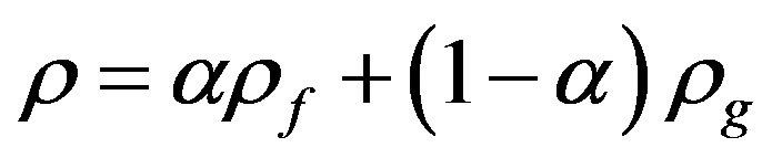
where:  is a velocity field suitable to compress the interface. The physical properties (µ and ρ) at any point in the domain are calculated as a weighted averaged of the volume fraction of the two fluids,
  , as:
, as:
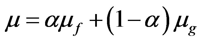 (11)
(11)
 (12)
(12)
2.3. Turbine Modelling
The IBF model is a compromise between at one extreme, a full treatment using overset meshing and/or sliding mesh techniques to describe the detailed internal blade motions and at the other, a highly simplified momentum extraction zone, such as the actuator disc method. For the IBF approach, a forcing function  is used representing the force applied by the immersed body (turbine) to the fluid to create momentum change and rotational flows. The forcing function can be defined as [9]:
 (13)
(13)
This forcing function was added in the NS equations as shown in (1) and a code was developed by considering drag and lift forces applied by the blades on the fluid flow as shown in Figure 1.
2.4. Computational Domain and Boundary Conditions
The computational domain shown in Figure 2 is a schematic representation of the dimensions of the geometry used for the computation. For simplification purposes of the computational domain and to minimise any pathymetry effect on the simulation results, the bottom of the domain was considered flat. The overall diameter of the turbine is D = 0.20 m. The domain size is 3D upstream of the turbine, 20D downstream, 11.1D width and with an overall height of 8.3D. Those dimensions were often used in the simulations but the width was subjected to some changes in the width proximity analysis.
Table 1 shows the number of cells used in the computational domain where the cell counts in the horizontal and vertical directions are represented by Nx and Ny respectively and along the span of the domain by Nz. The cell sizes are not the same throughout the domain in order to reduce the computational cost. The cell sizes were refined in the zone of interest around the turbine region in order to create a uniform computation. The grid topology and mesh are shown in Figure 3. The number of cells given in Table 1 was used for the computational domain given in Figure 2 but were changed based on the changes made on the domain dimensions for different analysis.
The computational domain contains seven boundary patches, namely atmosphere, seaBed, wall, water and air inlet and outlet. The top part of the domain was an atmosphere which represents a standard patch. This top boundary was free to the atmosphere and allows both outflow and inflow according to the internal flow. This was developed by a combination of pressure and velocity boundary conditions [11].
seaBed and wall are the floor and the front and back side of the computational domain respectively and both patches represent a wall. A zero Gradient boundary condition was applied to the pressure field.
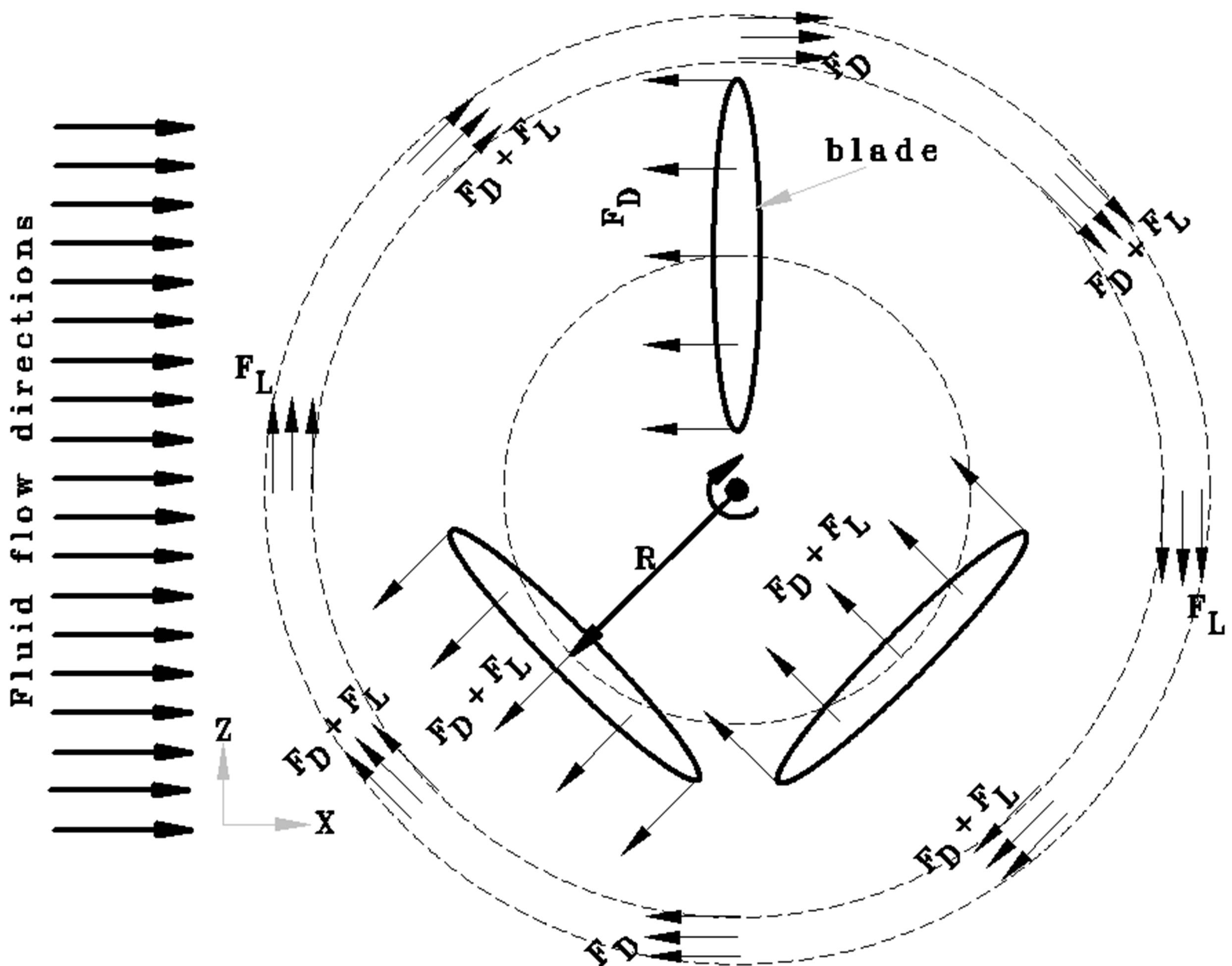
Figure 1. Schematic representation of the force directions of the IBF model.

Figure 2. Computational domain geometry.
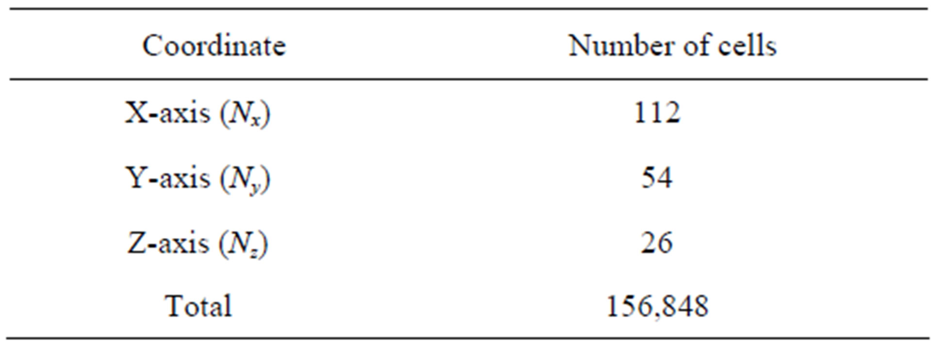
Table 1. Number of cells used for the computational domain.
In practical conditions, the velocity across the depth of a channel is often varied and has a parabolic velocity profile as described by [20-23]. Therefore, a parabolic velocity profile, which has been implemented by [11] and modified in this study to suit to a channel flow, was imposed on the inlet patch of the computational domain. Figure 4 shows the parabolic velocity profile extracted from the inlet boundary condition where the maximum velocity occurs slightly below the free surface (Y = 1.2625 m) similar to the arguments given by the number of authors discussed before. The velocity profile above the free surface shows zero velocity as expected because this region represents the air body of the computational. This inlet velocity profile has been used in the study of wake states of the MRL turbine by [9]. A maximum velocity of 0.746 m/s has been used for the simulations throughout this study.
3. Results and Discussions
3.1. Mesh Grid Size Sensitivity
Mesh grid size is an important factor in numerical simu-
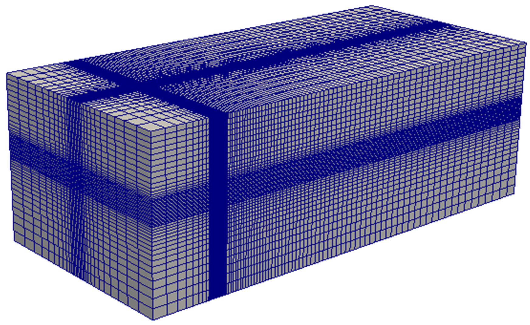
Figure 3. Non uniform mesh representation of the domain.
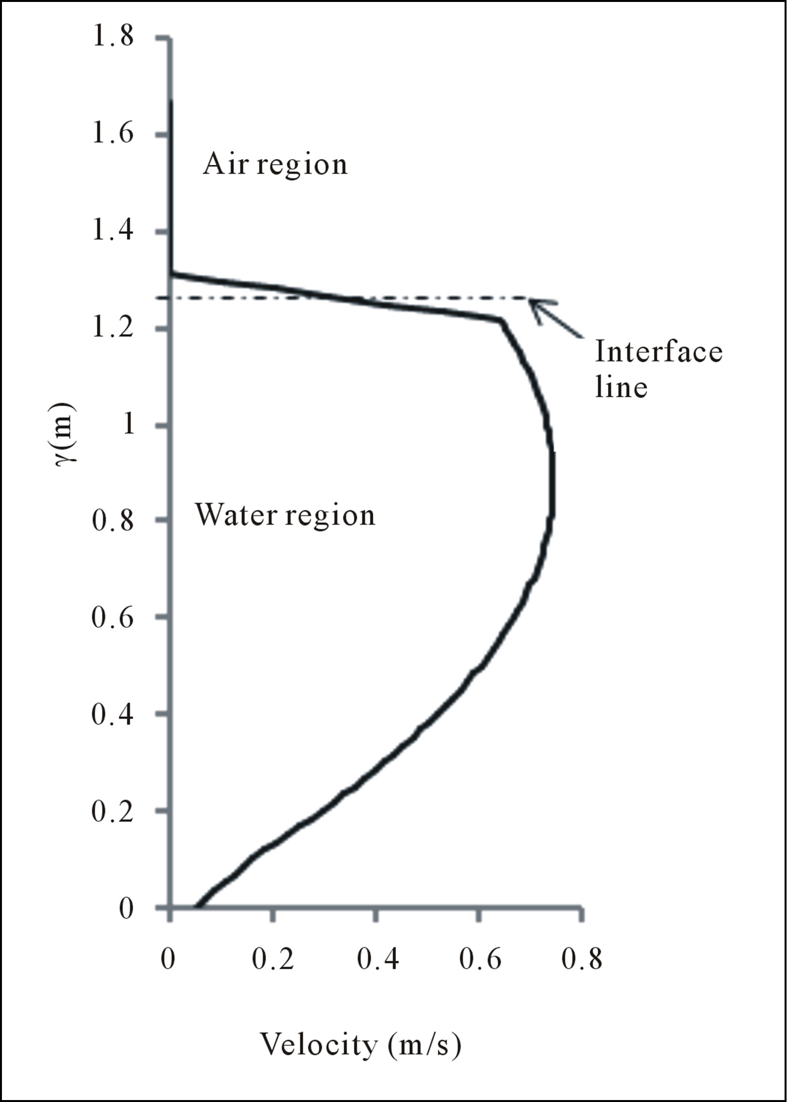
Figure 4. Non uniform mesh representation of the domain.
lations because resolving of the flow motions depends significantly on the grid size to accurately describe the flows. Thus, finding or developing the right model that can satisfy the engineering solutions without the need of fine grid size (cheap computational cost) is one of the biggest challenges engineers are facing nowadays. As the grid size gets finer, it inflicts a high computational cost because of the type of models used, such as the direct numerical simulation (DNS). In contrast, if the grid size gets coarser, this leads to use the models developed by approximations such as the Reynolds Average NavierStokes (RANS), which results poor description of the flow especially for the simulation of turbulent flows. Therefore, using the appropriate grid size is always crucial.
Three grid size samples (fine, medium, and coarse) have been chosen to investigate the grid size effect on the results as shown in Table 2. The grid size was refined in the zone of interest around the turbine region, in order to create uniform computation and increased towards both end of the domain to reduce the computational cost in the three cases.
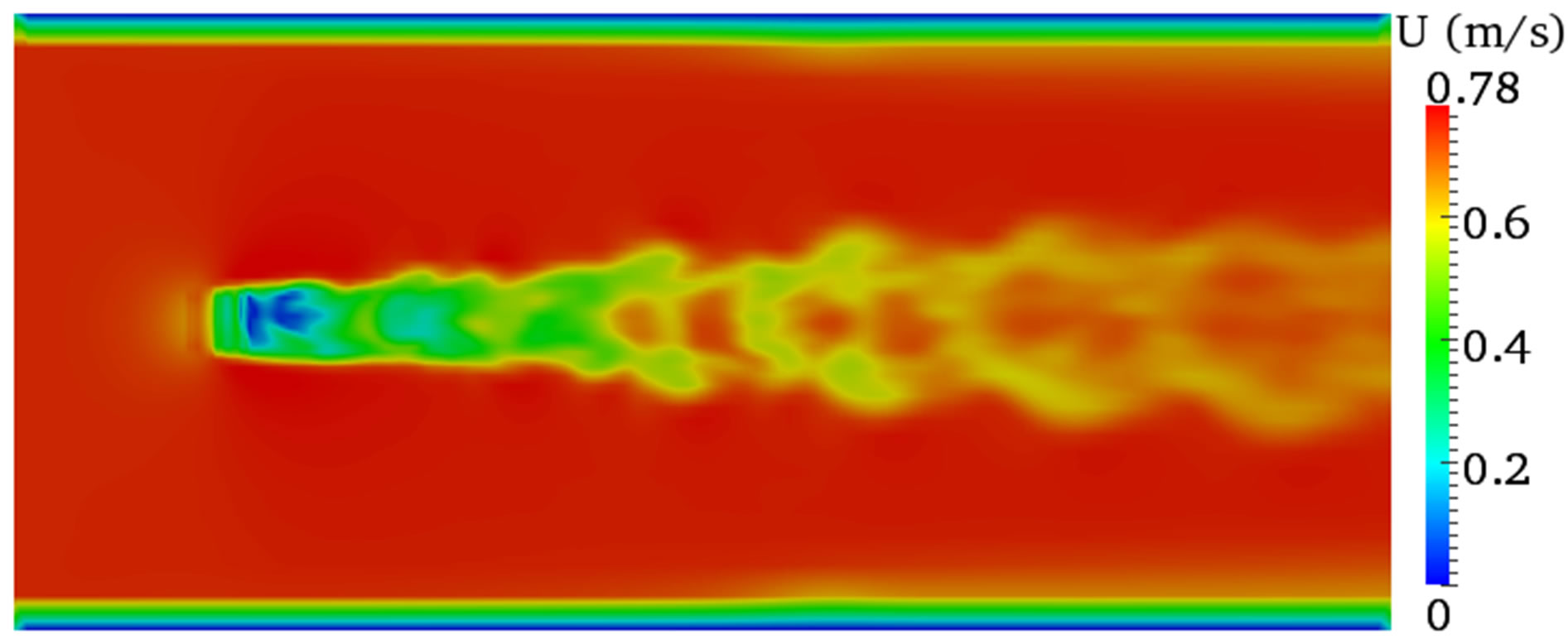
Figure 5 shows the velocity contours simulated with the three grid size samples. The results showed different flow features as expected. From the three grid sizes, the fine meshing (Figure 5(a)) showed clear distinction between the water and air body, which suggests to use fine grid size to adequately resolve the flow at the interface of the two phases. The fine grid size also reduced the boundary layer as the model properly resolved the flow at the interaction with the wall boundary as shown in Figure 5(b), which minimises the width proximity effect (see detail discussion about width proximity effect on section 3.2). In addition, it generated large scale vortexes downstream of the turbine and generally showed good flow descriptions.
However, the computational time was significantly increased compared with the other two meshing, which requires super-computing machines to minimise the time constraints and is not feasible.
In contrast, the results using the coarse grid size showed different flow characteristics (Figure 5(e)). More importantly, the result showed massive disturbances to the air body and makes it difficult to see a clear interface between the two phases. Thus, the CFD model is incapable of resolving the flow motions with coarse grid and requires fine grid to get proper description of the flows. However, the simulation result with the medium grid size produces satisfactory flow descriptions as shown in Figures 5(c) and (d). Therefore, the medium grid size is a good compromise between the fine and coarse grid sizes and therefore it is important to use the medium grid size throughout this study to minimise the long computational time inflicted by the fine grid size but satisfying the engineering solution.
3.2. Wall Boundary Proximity to the Turbine
Finding a proper proximity of the computational domain’s wall boundary to the MRL device is essential because of its influence on the simulation results in two ways. Firstly, the flow features will be affected due to the
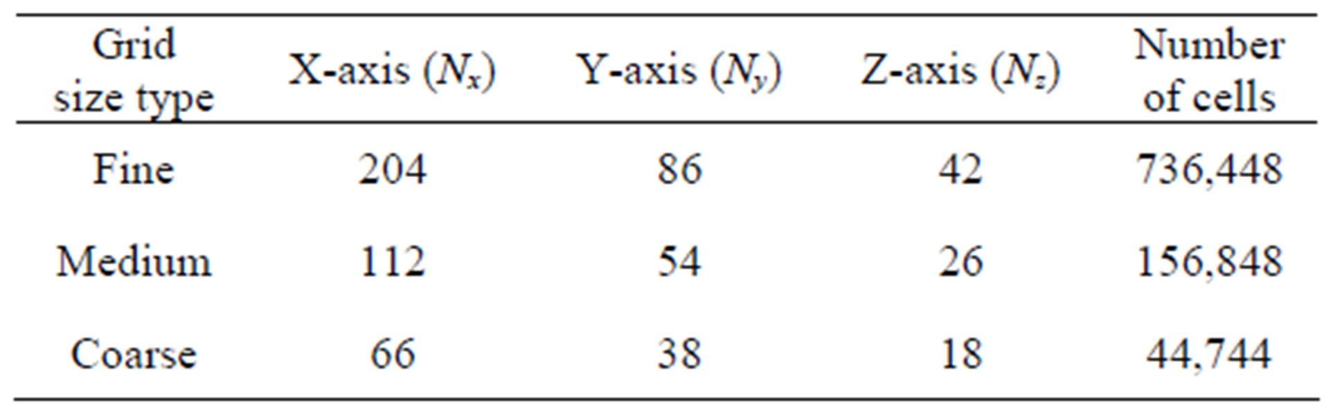
Table 2. Number of cells used for the three different grid sizes.
 (a)
(a)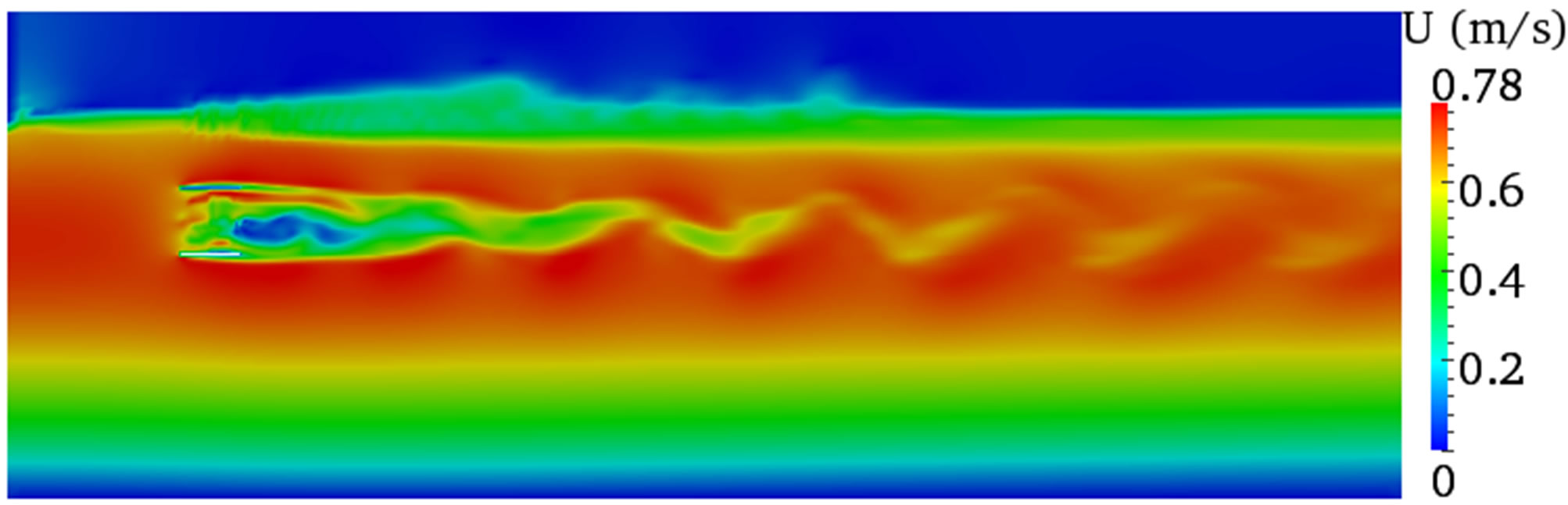 (b)
(b)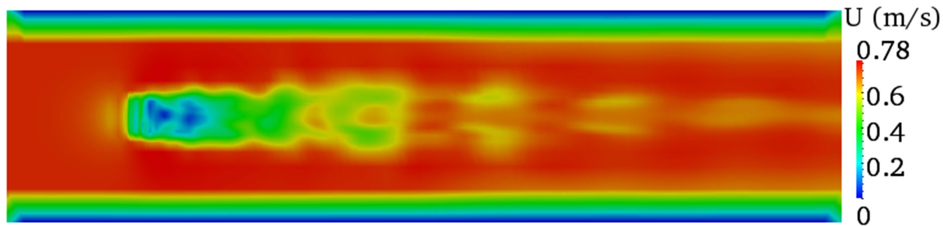 (c)
(c)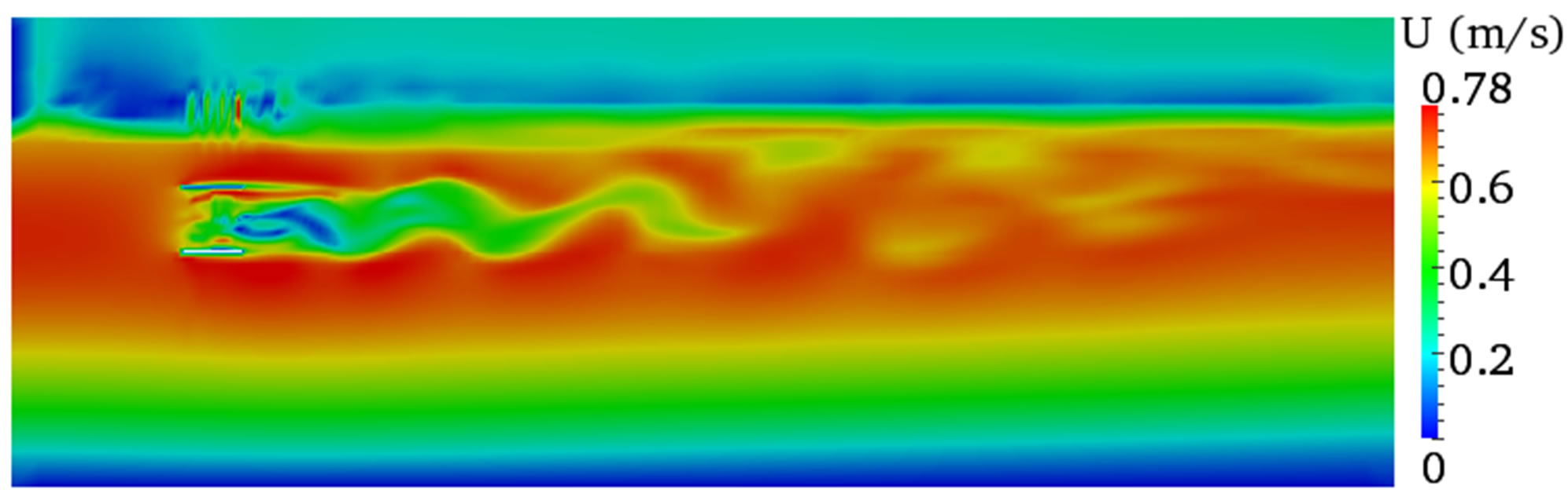 (d)
(d)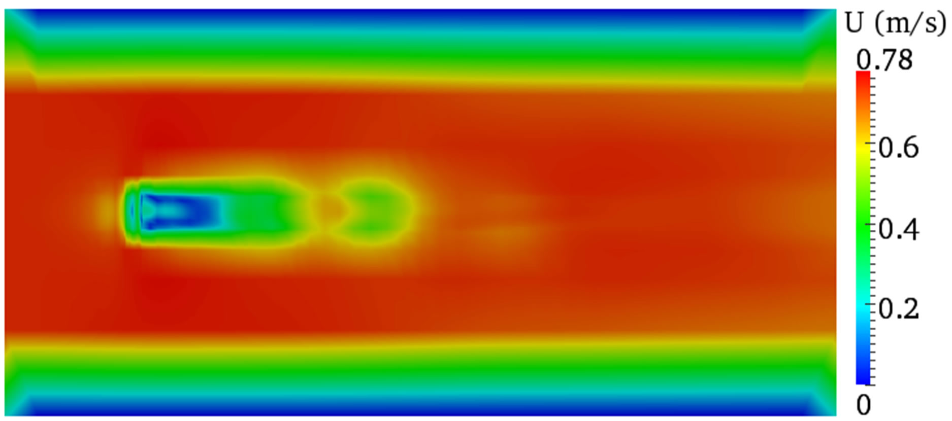 (e)
(e)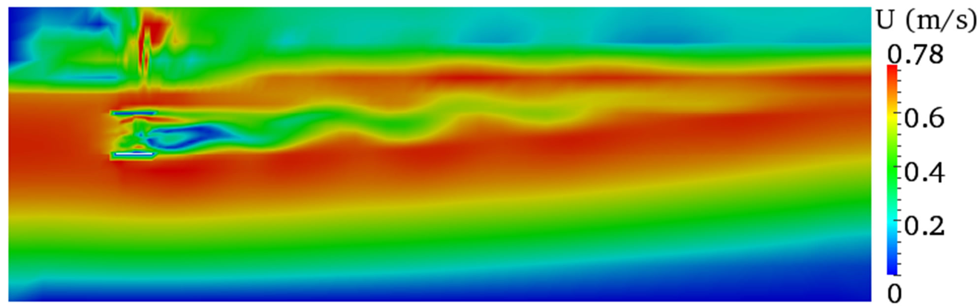 (f)
(f)
Figure 5. Velocity contours of different grid size. (a) Fine grid size vertical plane; (b) Fine grid size horizontal plane; (c) Medium grid size vertical plane; (d) Medium grid size horizontal plane; (e) Coarse grid size vertical plane; (f) Coarse grid size horizontal plane.
interaction of boundary layer with the turbine if small separation was to be used. Secondly, a large separation of the wall boundary and the turbine may inflict high computational cost. Therefore, to obtain an optimised width, three width dimensions (1.22 m, 2.22 m, and 4.22 m), which corresponds to the spacing between the wall boundary and turbine of 2.5D, 5D and 10D respectively on both sides of the turbine, were used for the analysis in this section. The medium grid size discussed in section 3.1 was used for the meshing but changed proportionately according to the width of the computational domain.
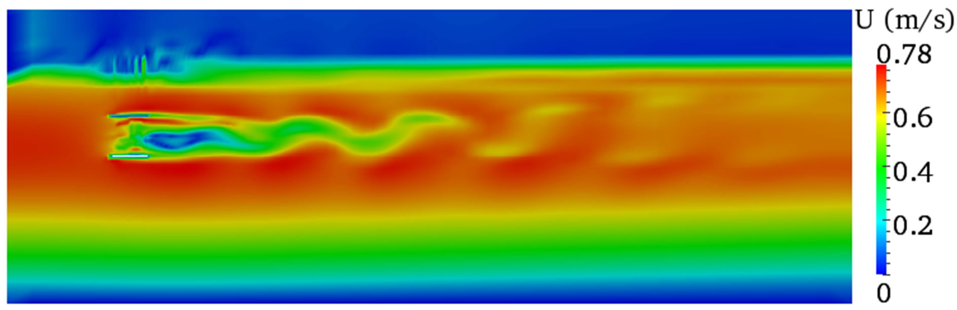
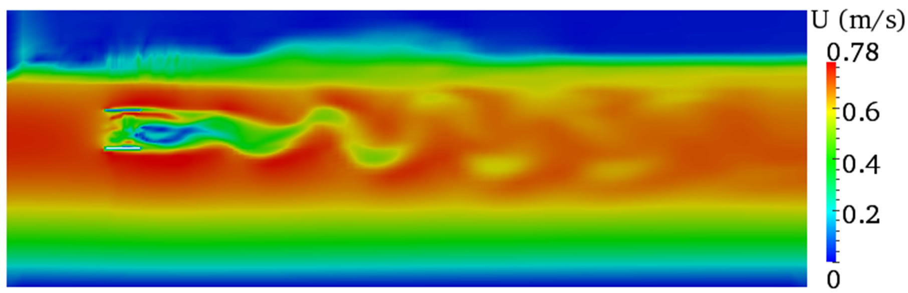
Figures 6-8 show the velocity contours both on the vertical and horizontal plane across the centre of the turbine. These results gave an insight of what happens to the flow features within and downstream of the turbine when the computational domain width is different. The simulation results showed different flow characteristics for the three domain widths used and these discrepancies were more visible on the vertical planes (Figures 6(a), 7(a), and 8(a)) at the interface between the two phases and on the air body.
The air body in the smaller width (W = 1.22 m) was severely affected leading to high velocity, which is not expected as the initial condition provided is zero velocity. However, the results from the other two width dimensions (W = 2.22 m and W = 4.22 m) showed clear difference between the two phases and the interface can be easily identified.
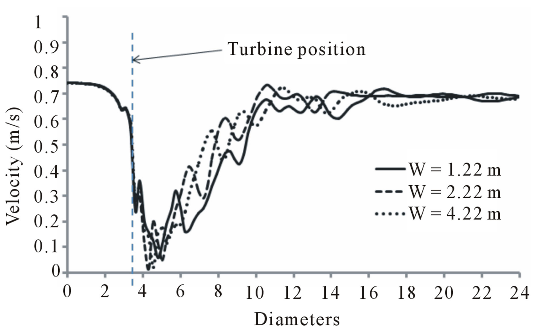
Figure 9(a) shows an instantaneous velocity profile extracted from the above velocity contours. The graph demonstrates that the velocity fluctuates immediately downstream of the turbine during the recovery process and sustains downstream up to around 14D. The fluctuation starts to vanish afterwards and showed almost smooth velocity profile. It seems difficult to differentiate the velocity profiles for the three width dimensions from this instantaneous velocity except a small difference observed between 6 and 8 diameters, where the wake showed slow wake recovery in the smaller width (W = 1.22 m). However, this is not always true as the velocity profile represents instantaneous value.
A time averaged velocity was then calculated to understand the difference of the actual wake recovery in the
 (a)
(a)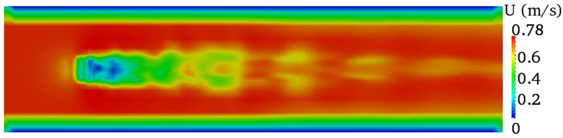 (b)
(b)
Figure 6. Velocity contours for a width of W = 1.22 m. (a) Vertical plane; (b) Horizontal plane.
 (a)
(a)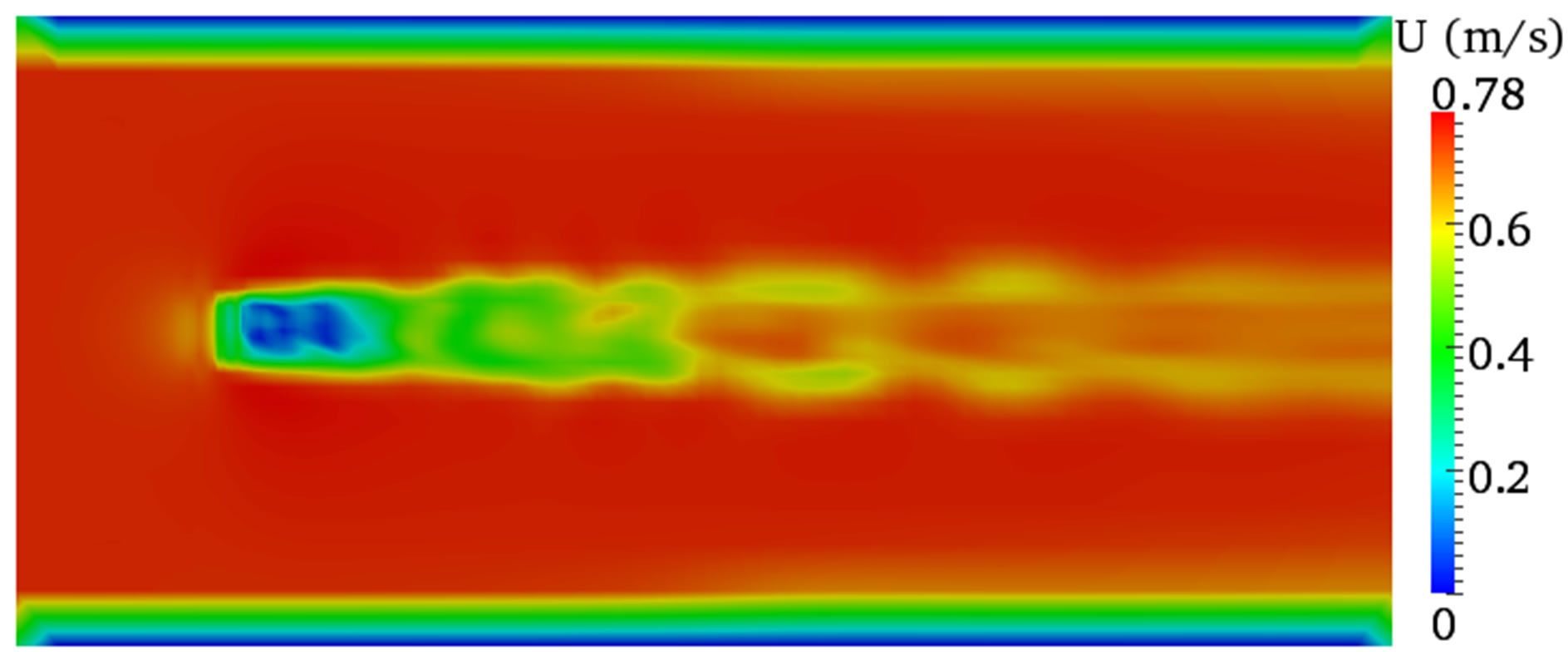 (b)
(b)
Figure 7. Velocity contours for a width of W = 2.22 m. (a) Vertical plane; (b) Horizontal plane.
 (a)
(a)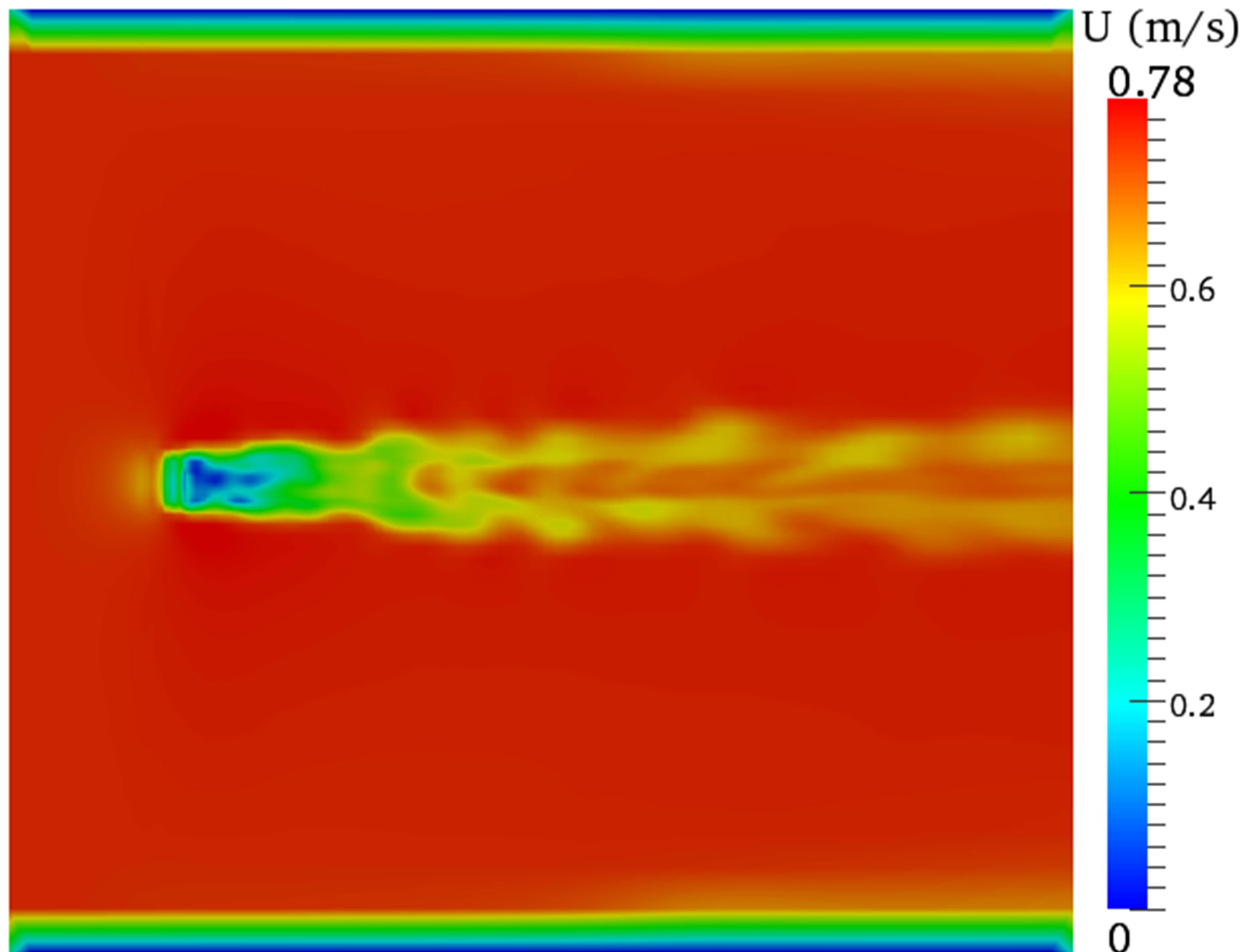 (b)
(b)
Figure 8. Velocity contours for a width of W = 4.22 m. (a) Vertical plane; (b) Horizontal plane.
 (a)
(a)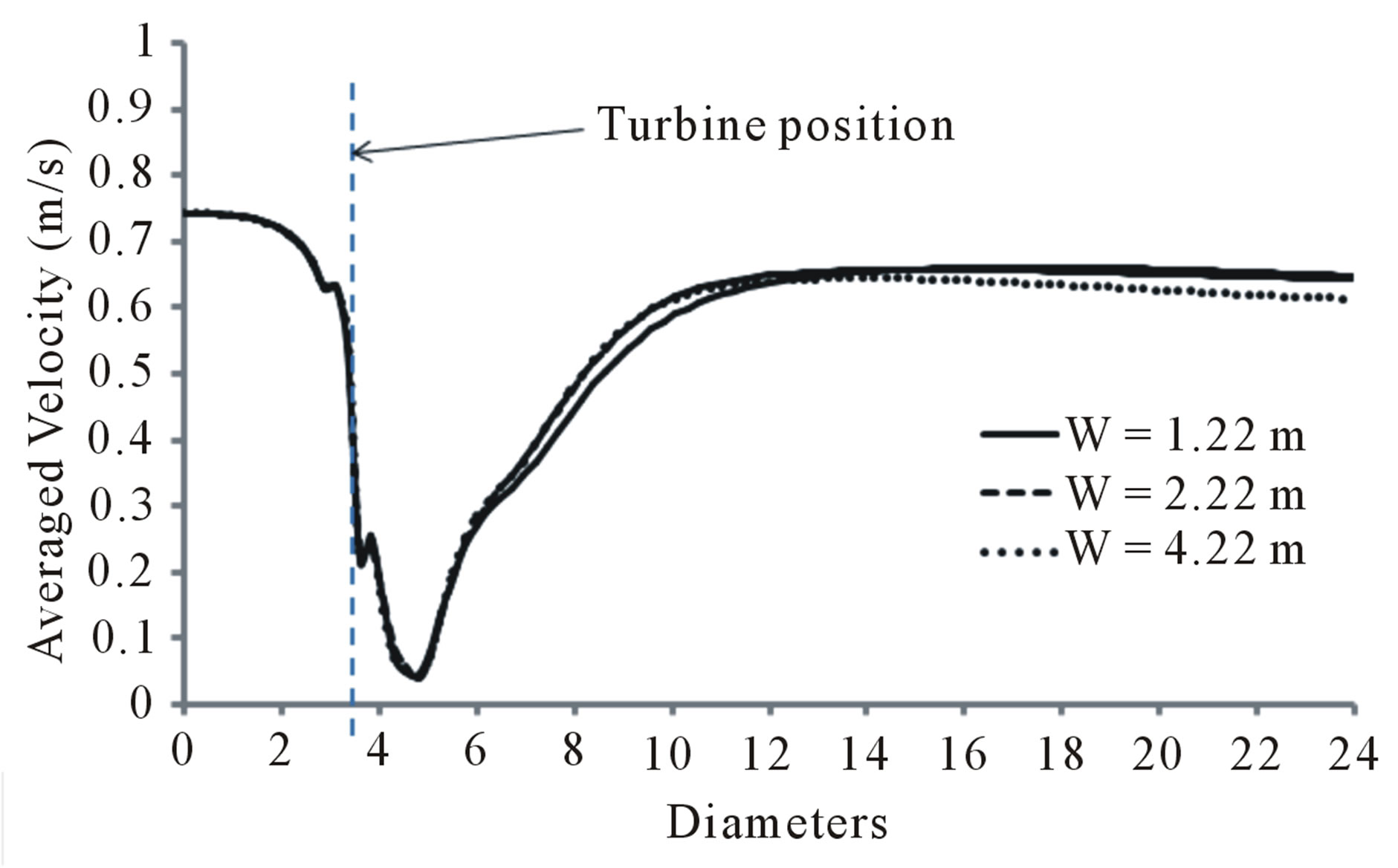 (b)
(b)
Figure 9. Stream-wise velocity profiles along the centreline of the turbine for the three domain width. (a) Instantaneous velocity; (b) Time average velocity.
 (a)
(a)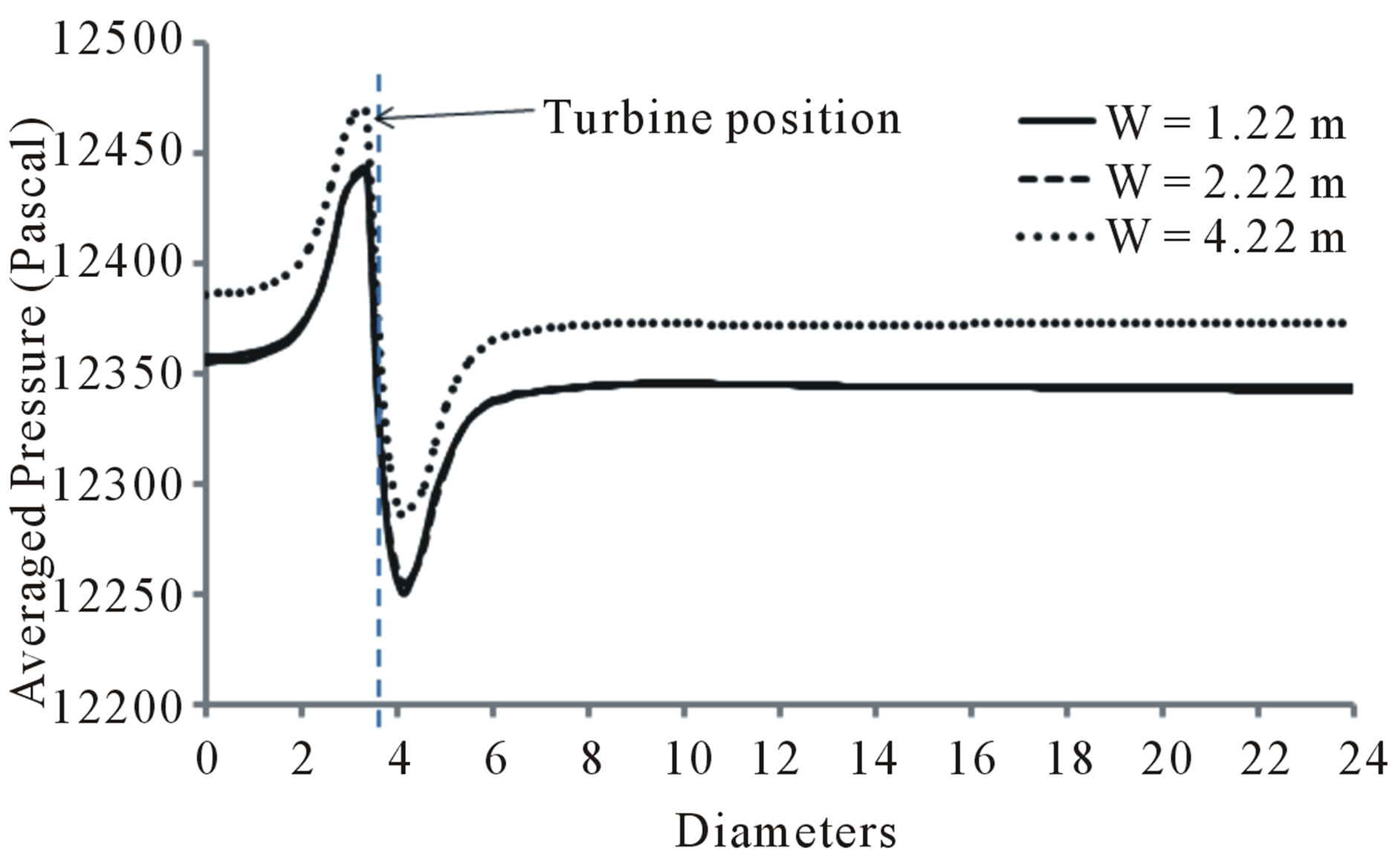 (b)
(b)
Figure 10. Stream-wise pressure profiles along the centreline of the turbine for the three domain width. (a) Instantaneous velocity; (b) Time average velocity.
three domains as shown in Figure 9(b). The fluctuations disappeared in the time averaged velocity profile and clearly showed the difference of the wake recovery among the three cases. The large width (W = 4.22 m) showed slower wake recovery compared to the other widths as shown at the end of the domain. This is mainly due to the reduction of the venturi effect of the computational domain’s wall boundary, which often accelerates the flow rate if a small width is used.
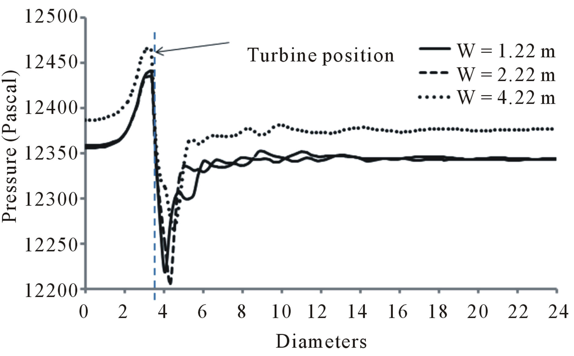
The pressure profile is another way of analysing the effect of the width domain as shown Figure 10. The results showed different pressure drop across the turbine using both the instantaneous and time averaged pressure profiles. However, in the case of the instantaneous pressure profile, there is still a pressure fluctuation, which reflects the velocity fluctuation discussed before. The turbine in the small width (W = 1.22 m) showed high pressure drop across the turbine region compared with the other two because of the venturi effect, which may lead to overestimate the power extraction by the turbine.
However, as the width increases the pressure drop decreases but at a slower rate. This indicates that with a very large width, the venture effect will be minimal. The pressure profiles in the smaller widths (W= 1.22 m and W = 2.22 m) were lower by almost 30 Pascal compared to the larger width due to the venturi effect, which drops the pressure by increasing the flow rate in the computational domain. Considering all the cons and pros, the turbine simulated in the medium domain width (2.22 m) would satisfy the necessary requirements of the simulation results. Thus, a computational domain which satisfies a domain width equivalent to around 5D spacing between the wall boundary and the turbine would be a potential choice.
4. Conclusions
The mesh grid size and width proximity have had massive impact on the simulation results, which can be summarised as follows:
• The fine meshing and the large width inflicted significant computational cost;
• The coarse meshing resulted poor description of the flow features because of the model used, which is unable to resolve the flow correctly with large grid size;
• Close proximity of the domain’s wall boundary to the turbine affected the free surface, the air body, and the flow characteristics at the interface between the two phases.
These results showed that careful investigation of the grid size requirement and the spacing between the wall boundary and the turbine is important to minimise the effects of these parameters on the simulation results. Generally, the results proved the capability of the IBF model in examining different tidal turbine issues.
5. Acknowledgements
MG Gebreslassie would like to thank for the financial assistance received from University of Exeter for this study.
REFERENCES
- R. Bedard, M. Previsic, O. Siddiqui, G. Hagerman and M. Robinson, “Survey and Characterization Tidal in Stream Energy Conversion (Tisec) Devices,” EPRI Final Report, 2005.
- G. Hagerman, B. Polagye, C. R. Bedard and M. Previsic, “Methodology for Estimating Tidal Current Energy Resources and Power Production by Tidal in-Stream Energy Conversion (TISEC) Devices,” 2006.
- B. Andrew, “Phase II Tidal Stream Energy Assessment,” Technical Report, 2005.
- S. Draper, G. T. Houlsby, M. L. G. Oldfield and A. G. L. Borthwick, “Modelling Tidal Energy Extraction in a Depthaveraged Coastal Domain,” Renewable Power Generation, Vol. 4, No. 6, 2010, pp. 545-554. Hdoi:10.1049/iet-rpg.2009.0196
- M. E. Harrison, W. M. J. Batten, L. E. Myers and A. S. Bahaj, “Comparison between CFD Simulations and Experiments for Predicting the Far Wake of Horizontal Axis Tidal Turbines,” Renewable Power Generation, Vol. 4, No. 6, 2010, pp. 613-627. Hdoi:10.1049/iet-rpg.2009.0193
- L. E. Myers and A. S. Bahaj, “Experimental Analysis of the Flow Field around Horizontal Axis Tidal Turbines by Use of Scale Mesh Disk Rotor Simulators,” Ocean Engineering, Vol. 37, No. 2-3, 2010, pp. 218-227. Hdoi:10.1016/j.oceaneng.2009.11.004
- S. Gant and T. Stallard, “Modelling a Tidal Turbine in Unsteady Flow,” Proceedings of the Eighteenth International Offshore and Polar Engineering Conference, 2008, pp. 473-479.
- X. Sun, J. P. Chick and I. G. Bryden, “Laboratory-Scale Simulation of Energy Extraction from Tidal Currents,” Renewable Energy, Vol. 33, No. 6, 2008, pp. 1267-1274. Hdoi:10.1016/j.renene.2007.06.018
- M. G. Gebreslassie, G. R. Tabor and M. R. Belmont, “CFD Simulations for Investigating the Wake States of a New Class of Tidal Turbine,” Journal of Renewable Energy and Power Quality, Vol. 10, No. 241, 2012.
- J. H. Ferziger and M. Peric, “Computational Methods for Fluid Dynamics,” Springer, Berlin, 1999.
- http://www.openfoam.com/docs/user/
- Z. Xie and I. P. Castro, “Les and Rans for Turbulent Flow over Arrays of Wall-Mounted Obstacles,” Flow, Turbulence and Combustion, Vol. 76, No. 3, 2006, pp. 291-312. Hdoi:10.1007/s10494-006-9018-6
- A. Leonard, “Energy Cascade in Large-Eddy Simulations of Turbulent Fluid Flows,” Advances in Geophysics, Vol. 18, 1975, pp. 237-248.
- A. Yoshizawa and K. Horiuti, “A Statistically-Derived Subgrid-Scale Kinetic Energy Model for the Large-Eddy Simulation of Turbulent Flows,” Journal of the Physical Society of Japan, Vol. 54, No. 8, 1985, pp. 2834-2839. Hdoi:10.1143/JPSJ.54.2834
- C. Yang, R. Lohner and H. Lu, “An Unstructuredgrid Based Volume-of-Fluid Method for Extreme Wave and Freely-Floating Structure Interactions,” Journal of Hydrodynamics, Vol. 18, No. 3, 2006, pp. 415-422.
- C. Yang, R. Lohner and S. C. Yim, “Development of a Cfd Simulation Method for Extreme Wave and Structure Interactions,” International Conference on Offshore Mechanics and Arctic Engineering (OMAE), Halkidiki, 2005.
- G. Chen, C. Kharif, S. Zaleski and J. Li, “Two Dimensional Navier-Stokes Simulation of Breaking Waves,” Physics of Fluids, Vol. 11, No. 1, 1999, p. 121. Hdoi:10.1063/1.869907
- X. He, S. Chen and R. Zhang, “A Lattice Boltzmann Scheme for Incompressible Multiphase Flow and Its Application in Simulation of Rayleigh-Taylor Instability,” Journal of Computational Physics, Vol. 152, No. 2, 1999, pp. 642-663. Hdoi:10.1006/jcph.1999.6257
- C. W. Hirt and B. D. Nichols, “Volume of Fluid (VOF) Method for the Dynamics of Free Boundaries,” Journal of Computational Physics, Vol. 39, No. 1, 1981, pp. 201- 225. Hdoi:10.1016/0021-9991(81)90145-5
- L. Gordon, “Mississippi River Discharge,” RD Instruments, San Diego, 1992.
- S. Q. Yang, S. K. Tan and S. Y. Lim, “Velocity Distribution and Dip-Phenomenon in Smooth Uniform Open Channel Flows,” Journal of Hydraulic Engineering, Vol. 130, No. 12, 2004, p. 1179. Hdoi:10.1061/(ASCE)0733-9429(2004)130:12(1179)
- M. H. Chaudhry, “Open-Channel Flow,” Springer Verlag, Berlin, 2008. Hdoi:10.1007/978-0-387-68648-6
- C. L. Chiu and N. C. Tung, “Maximum Velocity and Regularities in Open-Channel Flow,” Journal of Hydraulic Engineering, Vol. 128, No. 4, 2002, pp. 390-399. Hdoi:10.1061/(ASCE)0733-9429(2002)128:4(390)