Open Journal of Applied Sciences
Vol.3 No.1(2013), Article ID:29371,7 pages DOI:10.4236/ojapps.2013.31002
Estimating Circulation Patterns by Combining Velocity and Tracer Observations
1Department of Mathematics, University of Southern California Kaprielian Hall, Los Angeles, USA
2Naval Postgraduate School Moneterey, Monterey, USA
Email: piter@usc.edu
Received August 31, 2012; revised November 20, 2012; accepted November 29, 2012
Keywords: Data Fusion; Inverse Problem; Surface Velocities; Fuzzy Sets
ABSTRACT
A method is suggested for estimating unknown velocities by combining their sparse measurements with observations of a tracer on a fine grid advected by the underlined velocity field. The dependence of the estimation error on a coarseness parameter and parameters of the flow in question is investigated numerically using synthetic velocity fields typical for real oceanic circulation. In an advanced version of the estimation procedure uncertainty in the transport equation forcing is modeled via a fuzzy sets approach. We also compare the method with a traditional interpolation which is in contrast to the developed procedure unable to capture the flow details.
1. Introduction
The problem of retrieving a surface circulation in the ocean from observations of tracers such as sea surface temperature and chlorophyll concentration has been intensively discussed for the decades [1-15] because of its great practical and theoretical importance. In general it is an ill-posed inverse problem since the current component tangent to the tracer lines never can be recovered [2]. For that reason different additional conjectures were used to get a unique solution such as a scale separation [5-8]. In alternative approaches optimizing an appropriate cost function was suggested [3,4,13] or tracer observations were assimilated in numerical models of oceanic circulation [14].
If there is an independent source of information on the surface velocities such as a circulation model output then the problem can be formulated in a well-posed fashion using multi-objective optimization ideas [16-18]. The present work extends these ideas to a new set up which is of great practical importance: to estimate a surface circulation from high resolution tracer observations and sparse measurements of the surface velocity itself.
Typically, direct measurements of the surface velocities in the ocean covering a significant area cannot provide a high degree of the space resolution because of technical difficulties and high cost of such measurements. For example the distance between ADCP (Acoustic Doppler Current Profiler) stations in NAVOCEANO shipboard surveys (California Coastal Region) is about 18.5 km. On the other hand the space resolution of satellite observations of the sea surface temperature and chlorophyll concentration is much higher, 2 km or less depending on a type of radiometers. Thus, a task is to optimally combine these two kinds of data to restore the true circulation with highest possible resolution.
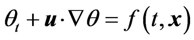
Here we consider a simplified formulation of the problem as follows. Assume that an unknown 2D velocity field  is observed on a coarse space grid
  at a fixed time
 . Then assume that two snapshots
  and
and  of a tracer field are available as well on a fine grid
 , where the tracer concentration is covered by
 (1)
(1)
with a poorly known forcing .
.
The problem is to estimate the velocity field on the fine grid by optimally combining both sorts of observations.
We first discuss the problem when the forcing in (1) is completely known (Section 2). This is the case for satellite observations of sea surface temperature since they are usually accompanied with heat fluxes measurements. In Section 3 we extend the approach to a poorly known forcing modeling its uncertainty in terms of fuzzy sets. An aimed area of application is the ocean color (chlorophyll). An estimation algorithm is derived for the corresponding two-objective fuzzy optimization problem. Numerical experiments with few types of synthetic flows typical for real oceanic circulation are presented in Section 4. Brief conclusions are summed up in Section 5.
2. Velocity Estimation under Completely Known Forcing
Let us fix a space point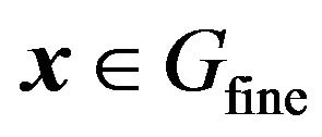 , time moment
  and assume
  and spacing
  of
of  to be small enough such that
  and
and  can be accurately computed.
Denote by  the velocities measured at
  nearest neighbors
  of x on the coarse grid
 . For the present purposes neither the number
  nor the configuration of the neighbors matters. To estimate the velocity
  at
at  we suggest to solve the following conditional optimization problem
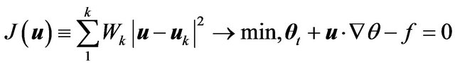
where  are prescribed weights (matrices or scalars). A quadratic cost function is traditionally used in statistical estimation problems. In our context its advantage is that unconditional optimization of
  leads to a linear interpolation widely used in oceanographic research.
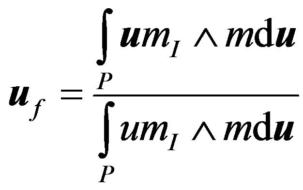
The solution obtained by a standard procedure of Lagrangian multiplier is given by
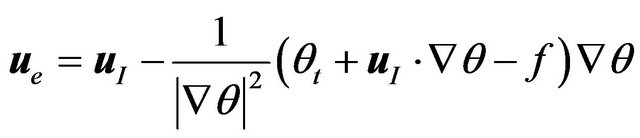 (2)
(2)
where
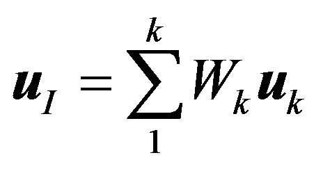 (3)
(3)
is the interpolated velocity. So, the resulting estimator consists of interpolation (the first term in (2)) and a correction according to the tracer observations (the second term).
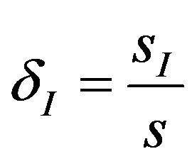
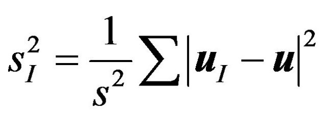
The estimation skill for each time moment we measure by the error ratio
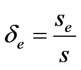
where
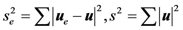
 is the true velocity and the summation is carried out over all the grid points in
 . The relative error
  will be compared to the interpolation error
where
Under some idealistic assumptions it can be shown similarly to [17] that
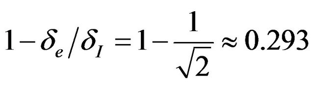 (4)
(4)
i.e. theoretically speaking the method would give about  improvement comparing to the interpolation. In our numerical experiments with realistic flows shown below this number varies in the range 12% - 32%.
3. Unknown Forcing
Here we assume that the forcing in (1) is not known, rather some reasonable confidence interval is available. Namely, one believes that
where  is a given background and
  is a margin depending on the location
  and moment
  as well which henceforth are fixed. The tracer gradient on the right hand side is introduced to keep the velocity dimension for
 .
.
Let us denote

then the last inequality is written as  where
where
To describe an uncertainty in knowledge of  we assume that
  is a fuzzy number with a membership function
  such that
  and
and  if
if  is outside of the interval
  [19,20]. To satisfy Equation (1) in condition of uncertainty about the forcing we formulate the problem of estimating
  as the following two-objective optimization problem
 (5)
(5)
which in the traditional approach does not have a solution in contrast to the conditional optimization discussed above for the case of known forcing.
A key concept in multi-objective optimization is a Pareto optimal solution, e.g. [21]. In plain words it is one in which any improvement of one objective function can be achieved only at the expense of another. For a formal definition see the cited paper.
To find the set  of all Pareto optimal solutions for (5) introduce
  for the interpolated velocity (3) and assume that
  is even and strictly increasing on
 , for example
  is a triangle membership function.
Direct computations lead to the following parametric description of 
 (6)
(6)
In other words,  is a segment on the straight line in the plane
  passing through
  perpendicular to the line
 . One of the endpoints of this segment is always coincides with
  given by (2) while the another one is either
  or
or  depending on whether
  is greater or less than
 .
.
In principle, any point from  could be treated as a sensible estimator of the true velocity. To single out a certain solution one can simply take the middle point of
 , however we suggest another way which is more consistent with fuzzy logic ideas and also allows to find out an explicit expression for the estimator. Namely, we change the set up (5) by replacing the quadratic cost function
  by an appropriate membership function
  centered at
  and then proceed to another fuzzy two-objective optimization problem
 (7)
(7)
In simple words we try to make the solution as close as possible to the interpolated velocity at the same time maximizing the possibility that just this solution advects the tracer.
The Pareto optimal set for (7) also can be efficiently described similarly to (6) and then the unique solution can be singled out by taking its center of mass
 (8)
(8)
according to fuzzy logic standard rules in aggregating information coming from different sources [19,20].
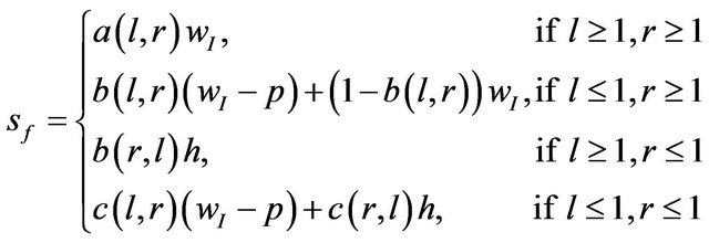
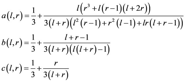
Let us parameterize 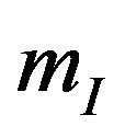 as a circular cone inside the circle
 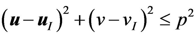 and zero otherwise where
  is a parameter characterizing uncertainties in the velocity observations. Then take
  as a triangle membership function defined by triplet
 . As a result (8) van be readily found in explicit form. Namely, denote
then (6) is expressible in form
 (9)
(9)
where for 
and for 
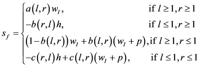
with
4. Simulations
4.1. Gyre Superimposed with Eddy System
In the first series of experiments the “true” velocity field is given by the following stream function
where
is the gyre with space scale  and the disturbing velocity is expressed by an oscillating regular system of eddies filling up the region

where  is the amplitude and
  is the fixed observation time. Finally, suppose that the initial tracer distribution is given by a Gaussian bell
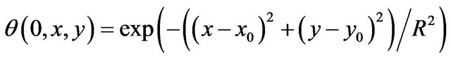
where R is the patch radius and  is its center.
In all below experiments the region  remains the same with
 . The fine grid
  defined as the set of all integer pairs
  is also kept constant (thus
 ), while the step of the coarse grid is defined by
  where
where  is the coarseness parameter which assumes three possible values
 .
.
4.1.1. Known Forcing
In the first experiment we assumed zero forcing for the tracer, . The estimates (2) were computed for each time moment
  with
with  and then compared to the pure interpolation.
Weights  in the interpolation objective function were chosen to be inversely proportional to the squared distances
  where x is the point in which the velocity is estimated and
  are vertices of the square in
  where
where  lies.
lies.
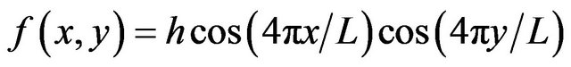
An example is shown in Figure 1 for the terminal time moment  under the following values of other parameters R = 10, Rb = 10, x0 = 3, y0 = 3, a = 5, k = 3, c = 8. As one can see, the estimated velocity field (first panel at the bottom) fairly captures principal features of the real velocity even for extremely high coarseness. In terms of numbers the relative estimation error
  is significantly less than the interpolation error
  such that
  which is well agreed with the theoretical bound (4).
We also show the gyre itself (last panel at the bottom) to illustrate that the interpolation itself captures well the large scale part of the circulation.
Results for other experiments are summarized in the following table.
From Table 1 the following conclusions can be drawn
- In all the instances the estimation error is less than the interpolation error.
- The estimation error is most sensitive to the coarseness parameter  characterizing sparseness of the velocity observations.
- The least influential parameter is the patch radius.
- The estimation error decreases as eddy density  decreases.
- As amplitude  kept constant, the range of improvement
  is
is  with the minimum value at
  and maximum value at
 .
.
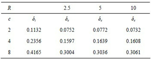
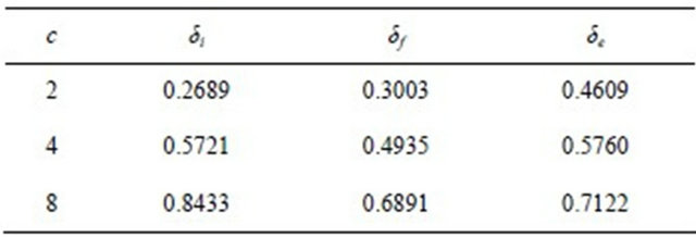
The goal of next two experiments whose results are presented in Tables 2 and 3 was to examine high and low amplitudes .
.
As one can see from Table 2 a sharp rise in the eddy amplitudes (ten times) modestly increases the estimation error, while when we go back to very small amplitude  the error decays by 2 - 3 times depending on the coarseness (Table 3).
4.1.2. Unknown Forcing
In the second series of experiments we tested the same model and “real” velocities with the “unknown” tracer forcing
 (10)
(10)
Real velocity fieid, k = 3, a = 5, c = 8 Observed veiocity field, k = 3, a = 5, c = 8 Tracer distribution under real velocity in 3 days
Esimated velocity field, k = 3, a = 5, c = 8 Optimal Interpolation, k = 3, a = 5, c = 8 Large scale velocity field, k = 3, a = 5, c = 8
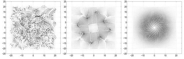
Figure 1. A gyre superimposed with a periodic eddy system: Upper panel: 1) “True” velocity; 2) Velocity observations; 3) Tracer observations. Bottom panel 1) Estimated velocity at ; 2) Interpolated velocity field; 3) Large scale component of the “real” velocity days.
Table 1. Dependence of the estimation and interpolation error on the eddy density (k), observation coarseness (c) and the patch radius (R) for the fixed amplitude a = 5.
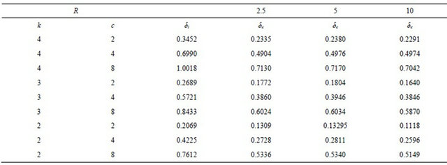
Table 2. Dependence of the estimation and interpolation error on the observation coarseness (c) and the patch radius (R) for the fixed amplitude a = 50 and eddy density k = 3.
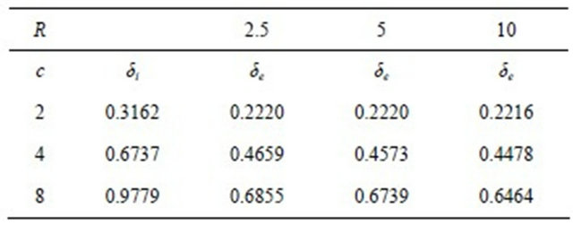
Table 3. Dependence of the estimation and interpolation error on the observation coarseness (c) and the patch radius (R) for the fixed amplitude a = 1 and eddy density k = 3.
where  is a given amplitude. The experiment conditions were the same as in the previous subsection except that the transport Equation (1) was integrated to generate tracer observations with the forcing given in (10) and the velocity estimates were obtained from the more general Equation (9) instead of (2). We underscore that in estimating the velocity field by (9) expression (10) for the forcing was not used at all. The only information on the forcing used for estimating was
  and
and .
.
The goal of experiments with fuzzy estimator (9) was to compare it with the estimator (2) which simply ignores the forcing uncertainty. We carried out such a comparison for two values of the parameter  characterizing the forcing intensity. The results are summed up in Tables 4 and 5. The relative error of the fuzzy estimator
  is defined similarly to
 .
.
The main conclusions concerning an unknown forcing are as follows:
- In most of scenarios the fuzzy estimator overperforms the non-fuzzy one.
- Under high amplitude of an unknown forcing and low coarseness the simple interpolation can perform better than either of the estimators.
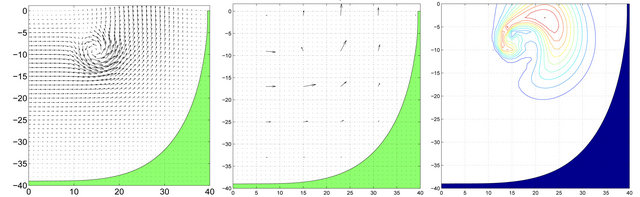
4.2. Coastal Flow
The goal of the last experiment Which is prensented in Figure 2 was to examine the method performance in detecting a single vortex (eddy) surrounded by a steady coastal current. The “true” velocity field is shown in the first panel at the upper row. On the next panel sparse direct velocity measurements are presented, which certainly do not allow to capture the eddy because of too low resolution. Finally, in the third panel we give tracer observations which exposing the eddy, but not sufficient to recover the whole flow.
The estimate according to the developed fuzzy algorithm is shown in the first panel of the lower row. One can see that the procedure was able to efficiently combine both kinds of the observations thereby adequately to retrieve both the eddy and background current. We compare the result with a pure interpolation (second panel) where the eddy turned out to be almost invisible. The only positive outcome of the interpolation is a fair estimate of the background flow (last panel).
In terms of numbers the improvement of the fuzzy estimate comparing to interpolation is only about , but in fact qualitatively the results are quite different.
5. Conclusions
A method is developed for estimating surface velocities on a fine grid by combining two kinds of observations:
True Observed velocity field Tracer
Estimated velocity field Optimal Interpolation Background

Figure 2. A synthetic coastal flow with an isolated eddy: Upper panel 1) “True” velocity. 1) Velocity observations; 2) Tracer observations; Bottom panel 1) Estimated velocity at t = 3 days; 2) Interpolated velocity field; 3) Large scale component of the “true” velocity.
Table 4. Comparison between the fuzzy estimator (δf), non-fuzzy (δe, Section 2), and interpolation (δi) for h = 5.
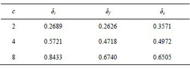
Table 5. Comparison between the fuzzy estimator (δf), non-fuzzy (δe, Section 2), and interpolation (δi) for h = 10.
velocity itself on a coarse grid and tracer on a fine grid.
The first version of the method is aimed at the known forcing in the transport equation. The corresponding estimator is nothing more but the solution of a classical conditional optimization problem with a traditional quadratic cost function. Numerical experiments were conducted with a gyre superimposed by a vortex system to investigate the method performance depending on the coarseness of velocity measurements, the number of eddies, and the gyre radius. Improvement in the estimate comparing to the pure interpolation was around 25% - 40% depending on the above parameters.
In the second version of the method designed for a poorly known forcing we model uncertainties in the forcing and velocity measurements using a fuzzy set approach. Arising a simple two-objective fuzzy optimization problem allows an explicit solution. With poorly known forcing an improvement in estimation comparing to interpolation is more modest. Moreover, for low coarseness interpolation can work even slightly better under large unknown forcing. As for comparing the fuzzy and non-fuzzy algorithm (which does not account for uncertainties in the forcing at all) the former is better in all the scenarii, even though the difference in estimation error is not much significant.
On the qualitative level the method overperforms interpolation as well for a typical coastal flow with an isolated eddy.
6. Acknowledgements
The support of the Office of Naval Research under grant N00014-11-1-0369 and NSF under grant CMG-0530893 is greatly appreciated.
REFERENCES
- C. Wunsch, “The North Atlantic General Circulation West of 50W Determined by Inverse Methods,” Reviews of Geophysics, Vol. 16, No. 4, 1978, pp. 583-620. doi:10.1029/RG016i004p00583
- M. E. Fiadeiro and G. Veronis, “Obtaining Velocities from Tracer Distributions,” Journal of Physical Oceanography, Vol. 14, No. 11, 1984, pp. 1734-1746. doi:10.1175/1520-0485(1984)014<1734:OVFTD>2.0.CO;2
- C. Wunsch, “Can a Tracer Field Be Inverted for Velocity?” Journal of Physical Oceanography, Vol. 15, No. 11, 1985, pp. 1521-1531. doi:10.1175/1520-0485(1985)015<1521:CATFBI>2.0.CO;2
- K. A. Kelly, “An Inverse Model for Near-Surface Velocity from Infrared Images,” Journal of Physical Oceanography, Vol. 19, No. 12, 1989, pp. 1845-1864. doi:10.1175/1520-0485(1989)019<1845:AIMFNS>2.0.CO;2
- C. Frankignoul and R. W. Reynolds, “Testing a Dynamical Model for Mid-Latitude Sea Surface Temperature Anomalies,” Journal of Physical Oceanography, Vol. 13, No. 7, 1983, pp. 1131-1145. doi:10.1175/1520-0485(1983)013<1131:TADMFM>2.0.CO;2
- A. G. Ostrovskii and L. I. Piterbarg, “Inversion for the Heat Anomaly Transport from SST Time Series,” Journal of Geophysical Research: Oceans, Vol. 100, No. C3, 1995, pp. 4845-4865. doi:10.1029/94JC03041
- A. G. Ostrovskii and L. I. Piterbarg, “A New Method for Obtaining Velocity and Mixing Coefficients from Time Dependent Distributions of Tracer,” Journal of Computational Physics, Vol. 133, No. 2, 1997, pp. 340-360. doi:10.1006/jcph.1997.5674
- A. G. Ostrovskii and L. I. Piterbarg, “Inversion of Upper Ocean Temperature Time Series for Entrainment, Advection, and Diffusivity,” Journal of Physical Oceanography, Vol. 72, No. 1, 2000, pp. 301-315.
- W. J. Emery, A. C. Thomas, M. J. Collins,W. R. Crawford and D. L. Mackas, “An Objective Procedure to Compute Surface Advective Velocities from Sequential Infrared Satellite Images,” Journal of Geophysical Research, Vol. 91, No. 12, 1986, pp. 12865-12879. doi:10.1029/JC091iC11p12865
- W. J. Emery, C. W. Fowler and C. A. Clayson, “Satellite Image Derived Gulf Stream Currents,” Journal of Atmospheric and Oceanic Technology, Vol. 9, No. 3, 1992, pp. 285-304.
- I. Crocker, D. Matthews, W. J. Emery and D. Baldwin, “Computing Ocean Surface Currents from Infrared and Ocean Color Imagery,” IEEE Transactions on Geoscience and Remote Sensing, Vol. 45, No. 2, 2007, pp. 435- 447. doi:10.1109/TGRS.2006.883461
- A. Turiel, J. Sol, V. Nieves, J. Ballabrera-Poy and E. Garca-Ladona, “Tracking Oceanic Currents by Singularity Analysis of Microwave Sea Surface Temperature Images,” Remote Sensing of Environment, Vol. 112, No. 5, 2008, pp. 2246-2260. doi:10.1016/j.rse.2007.10.007
- A. F. Bennett, “Inverse Methods in Physical Oceanography,” Cambridge University Press, Cambridge, 1992. doi:10.1017/CBO9780511600807
- E. Huot, T. Isambert, I. Herlin, J.-P. Berroir and G. Korotaev, “Data Assimilation of Satellite Images within an Oceanographic Circulation Model,” Acoustics, Speech and Signal Processing, Vol. 2, No. 3, 2006, pp. 265-268.
- W. Chen, “Nonlinear Inverse Model for Velocity Estimation from Infrared Image Sequences,” International Archives of the Photogrammetry, Remote Sensing and Spatial Information Science, Vol. 8, No. 10, 2010, pp. 958- 963.
- A. Mercatini, A. Griffa, L. Piterbarg, E. Zambianchi and M. G. Magaldi, “Estimating Surface Velocities from Satellite Data and Numerical Models: Implementation and Testing of a New Simple Method,” Ocean Modeling, Vol. 33, 2010, pp. 190-203. doi:10.1016/j.ocemod.2010.01.003
- L. I. Piterbarg, “A Simple Method for Computing Velocities from Tracer Observations and a Model Output,” Applied Mathematical Modeling, Vol. 33, No. 1-2, 2009, pp. 3693-3704. doi:10.1016/j.apm.2008.12.006
- L. I. Piterbarg and L. Ivanov, “Fuzzy-logic Based Algorithm for Estimating Circulation Patterns,” Current Applied Mathematics, Vol. 1, No. 1, 2011, pp. 17-39.
- D. Dubious and H. Prade, “Possibility Theory,” Plenum Press, New York and London, 1986.
- G. Shafer, “A Mathematical Theory of Evidence,” Princeton University Press, Princeton, 1976.
- K. Deb, “Multi-Objective Optimization Using Evolutionary Algorithms,” Willey, Hoboken, 2001.