
Advances in Linear Algebra & Matrix Theory
Vol.04 No.01(2014), Article ID:43474,30 pages
10.4236/alamt.2014.41002
The Better Accuracy of Strassen-Winograd Algorithms (FastMMW)
Paolo D’Alberto
FastMMW, San Jose, USA
Email: paolo@fastmmw.com
Copyright © 2014 by author and Scientific Research Publishing Inc.
This work is licensed under the Creative Commons Attribution International License (CC BY).
http://creativecommons.org/licenses/by/4.0/



Received 2 January 2014; revised 10 February 2014; accepted 17 February 2014
ABSTRACT
The first error theory and bounds for Fast Matrix Multiplication based on the Strassen-Winograd algorithms (FastMMW) were formulated in the 70s. The theory introduces the concept, which is now known as weakly-stable error analysis, where the error bounds must use matrix norms instead of component-wise bounds. While the theory debunked the instability myth by using matrix scaling and a clean and simple analysis, its bounds are available only as properties of the whole matrices, which are too coarse, pessimistic, at times used to suggest instability, and are not used for algorithm optimization. We build on top of the original theory in order to reformulate the bounds: we show that tighter norm-wise and component-wise bounds are achievable by orthogonal algorithm optimizations. To achieve even better discrimination and circumvent the use of norm bounds, we develop an error theory by using communication and statistics concepts: we investigate lower and upper bounds, we estimate the practical bounds, and we investigate the algorithmic nature of the error for the class of random matrices. The theory and tools are not limited to random matrices and we can foresee further investigations to different matrix classes and algorithms. We propose new and more accurate algorithms. We show that we can improve theoretically and empirically the maximum absolute error of any FastMMW algorithm by 10% - 20% per recursion (we reduce the error by half for 4 recursions). Our theory and practice, in turn, will provide a kick start for the development of hybrid algorithms as accurate as the vendor GEMM implementation, and in certain cases even more accurate for random matrices.
Keywords:
Matrix Multiplications; Algorithms; Performance; Error Analysis

1. Introduction
We are interested in the analysis, design, and implementation of the algorithms known as Fast Matrix-Multipli- cation based on the variants of Strassen and Winograd (i.e., Fast Matrix Multiplication by Winograd’s algorithms FastMMW see [1] [2] based on bilinear technique). We are drawn towards these algorithms because of their beauty, performance advantages, and, here we address a novel theory and measures to resolve the ever- present concerns about numerical stability and practical use of the FastMMW. We argue that the theory and the tools available are basically unchanged since their introduction forty years ago probably because these bounds have been used to discourage the use of the FastMMW, with a few exceptions [3] [4] . Here, we improve those bounds by more accurate algorithms and we introduce new tools.
The FastMMWs are used and investigated in several contexts, there is a wealth of related work; furthermore, with every new architecture there are new implementations, and thus new results. For example, we have a small contribution in the exploration of a large set of architectures. In practice, performance is the main reason for the FastMMW proposal and we often hear that accuracy is the main concern. Here, we address the accuracy of the FastMMW for any type of matrices and we provide new tools to handle the class of matrices broadly called random.
We show that using the theory developed by Brent [5] , Miller [6] , and Bini and Lotti [7] , we can design bilinear algorithms (thus Strassen-Winograd variants) that are more accurate than what was known. The theory will provide the tools so that we can estimate the accuracy gain a priori and for any algorithm. These bounds are still based on the theory of weak-stability and thus on norm wise bounds. These bounds provide an estimate of the maximum error for the whole computation, the whole result matrix. These bounds provide quite an over estimate for most of the result matrix component because they do not offer appropriate component-wise bounds. This is a practical and important concern that we will address in the following and present evidence for random matrices.
In our work, the design of kernel algorithms, we struggle in providing performance and accuracy estimates for our algorithms. We struggle because we do not always know the context where our algorithms will be applied. The application of random matrices for such estimates is common. Random matrices are useful tools to describe the range (i.e., in the range [0, 1]) and the values of matrices without a clear pattern (e.g., with normal distribution); that is, random. This class of matrices is special: they have full rank and they are dense. Being without pattern makes them a little remote to be a benchmark, in the common sense of the term; however, they are ideal for the testing of algorithms. There are a few good reasons why researchers, like us, entertain the testing with these special matrices, in the following we share three.
First, there is a known unknown effect. If we design a new algorithm and we want to test its performance and accuracy, it is plainly impossible to test every possible matrix. We know that we do not know what matrices will be used, so we substitute our unknown matrices with something random. It is an understandable and common misdemeanor.
Second, there is a practical appeal. They are easy to generate with different statistical properties: uniformly distributed in an interval such as [−1, 1] or Normal with specific mean and variance just to give two common continuous distributions (e.g., a user-guide of random matrix [8] as suggested by a reviewer). Here, the absence of a pattern or random as by Kolmogorov [9] should be associated with the error committed during the computation; however, the simplest way is to control the random nature of the input matrices1. The absence of a pattern assures the testing of every instruction and its contribution to the output. The independent and weighted, accordingly to importance, contribution of each instruction is the ultimate reward. Often, the former helps bring forward the latter. Nonetheless, these matrices are non-singular with probability one and thus they may avoid important corner cases in the context of matrix factorization.
Third, there is a statistical appeal. We know and we control the statistical features of the input and we measure the statistical properties of the output quite easily. We can use such information to derive the so called transfer function for the algorithms; we provide a formal definition starting from Section 4. The random matrix is a tool for the computation of the transfer function. If we obtain an adequate transfer function, we can estimate statistical properties of the output. Among these properties, there are also the distribution range of the maximum absolute error and its location in result matrix: the maximum error is the most common measure to estimate the accuracy of an algorithm. We are interested in a component-wise transfer function so as to estimate component-wise error bounds.
The transfer function has specific properties that will allow us to extend the weak-stability error analysis and our optimizations to random matrices and to obtain component-wise bounds.
We can state our contribution in one paragraph. Here, we present a methodology that will improve the FastMMW error bounds and will provide the estimate and measure of the error for each component of the result matrix for random matrices. This allows us to have a complete error-analysis tool set: we shall model the error, measure the error (by experiments in floating point arithmetic in IEEE-754 single precision floating point arithmetic), validate the model, and ultimately we shall design and implement more accurate algorithms. These algorithms enrich the FastMMW software package. In turn, all performance tables, plots, and other graphical presentations are drawn automatically using the Python FastMMW package. The self-contained software will help any independent validation and reproduction of all the following results: ultimately, it will simplify the exploration of new algorithms in the future and the transfer of FastMM algorithms to a larger audience.
We organize the paper as follows: in Section 2, we introduce the theory of weak stability, that is, the most successful error analysis as of today with the relative references, a description of the main ideas and our main difference. In Section 3, we bridge together the error analysis with tools used in linear time-series analysis. In Section 4, we introduce and formalize the transfer function. We present a complexity analysis using transfer function in Section 5. Using this analysis, we propose optimizations in Section 6. In Section 7, we show the practical relation between the transfer-function complexity and the weak stability. We draw our conclusions in Section 8.
2. Weak Stability
Obviously, an algorithm is a constructive way of representing and computing a function. The output of an algorithm is often an approximation to the true result due to the approximation of the data and of intermediary states of the computation. Stability analysis is the ability to quantify the maximum or the expected error an algorithm will introduce during and at the end of its computation.
The most natural way to quantify an error is by estimating the difference between what we should compute and what we compute instead. So if the ideal computation with ideal representation of the inputs and outputs is a matrix  then we will represent the computed values as
 . Of course, the
  Matrix Multiplication is
simply the computation  (where even the input matrices
  and
and  may be affected by an
initial error).
The component-wise comparison between  and
and  is
is

This is a matrix representing the absolute difference of the two matrices and the equality is meant to be component wise  where
where  represents the row and
  the column of the matrices,
 .
.
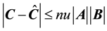
We know that for any Matrix Multiplication (MM) using  operations the error is:
 (1)
(1)
The interpretation is simple and important. Given any component error , this is bounded from above by the size of the matrices
 , by the precision of the hardware
 , and by the absolute value of the operands
 ; that is the dot product of i-th
  row and the j-th
  column (i.e.,
 ). In fact, each component error has the same bounds because the result matrix is the computation of
  independent dot products. The bound is a function of
  because it involves
  additions (and
  multiplications):
  re- presents the maximum addition-chain length and how the error at the beginning of the chain will carry on to the end. Finally, the hardware data representation uses a format that has unit roundoff,
  , which means that in absolute terms the error is larger for large numbers and thus for arithmetic with large numbers.
The first bounds for the FastMM accuracy are by Brent [5] . He studied the Winograd algorithm [10] , where the inner product can be organized to save one half of the scalar multiplication, and Strassen’s recursive algorithm, with 7 recursive MM and 18 matrix additions [1] . Brent has proposed a specific bound for Strassen’s like algorithms. After forty years, these are the de facto best bounds, which define the error bounds for FastMM. We re-state here Brent’s bounds again and provide an intuitive meaning.
For both Strassen’s and Winograd’s (for the latter Higham provides a complete analysis [11] [12] Chapter 23, Theorem 23.3 where he traces back the recurrence equations and solutions) like algorithms:
 (2)
(2)
Where  is the recursion point where the fast algorithm yields to the general MM or leaf computation. The constant
  is a function of the algorithm; for Strassen’s 18 addition algorithm
 , whereas Winograd’s 15 addition algorithm
 . Here, the estimate is not a matrix but a real number. With the notation
 , we identify the norm operation, here and, in the literature is called max norm, defined as

Intuitively, the ratio  is the number of recursion steps from the original problem size
  to
to . The
. The
Factor  is a function of the longest path of additions (i.e., matrix additions) within a recursion step of the algorithm.
Without loss of generality and to simplify the equation, consider the matrices unitary so that
 (i.e., by scaling) and we can neglect the factor
  because it is an architecture feature and not an algorithm feature. Thus we can turn our attention on the two important ideas of this equation: First, the error is a function of the leaf computation (i.e., error at the leaf); second, the error we commit is a multiplicative factor of the leaf error: in particular as a function of the number of recursion levels
 .
.
For example, for one level of recursion,  , we can estimate a multiplicative factor of
  to the leaf error. In practice, for
  level of recursions in the worst case scenario we should have a multiplicative factor of
  (or
(or  for Winograd). The best case scenario is for
 , the shortest addition chain, and thus the factor is just
 . This means that the error will be linear as function of the problem size (
 where
where  is a constant parameter).
We understand from this equation that we can apply two different optimizations: we improve the leaf computation [13] [14] or we decrease the length of addition chains [7] . We investigated the former approach, for the latter Bini and Lotti present a Winograd algorithm with  (unfortunately, with no implementation nor experiments). In this work, we show a third approach: by reducing the catastrophic effects of long chains.
Miller [6] showed that the estimate of Equation (1) cannot be applied to FastMM because part of the result matrix has different bounds (e.g., not uniform). What he proposed is to use a norm-wise bound that should follow this form:
 (3)
(3)
Miller infers that Brent’s bound are the best we can infer for FastMM because Equation (2) satisfies the form of Equation (3). In practice, Miller argument is to introduce and evaluate different ways to compute bounds for bilinear forms (FastMM) and he introduces the terminology known today: Brent stability and Restricted Brent stability (in honor to the original author) and the more common term of Weak and Strong Stability. In the literature and in this paper, we mean the weak stability as the Brent Stability (norm wise bounds).
In Section 4, we shall present graphical tools and bounds that will make obvious Miller’s error bounds [6] . In short and intuitively, the  for FastMM are not independent; the algorithm will focus on, for the lack of a better term, the error in specific locations of the matrix. We can provide point wise bounds satisfying Miller’s bounds and providing an optimization tool, thus we can develop more accurate FastMM algorithms.
Bini and Lotti [7] provide the first framework to describe by recurrence equations the error of any bilinear algorithms, which are expressed by matrices and matrix products. Their idea is to keep separated the (block) error that will affect the  and they split the matrix error into quadrants.
 (4)
(4)
They estimate the error as a multiplicative factor for each quadrant but they do not care about their order. They define it stability vector and we represent the error location by means of a matrix:
 (5)
(5)
The component/matrix  is the maximum error associated with component/quadrant
 .
.
This is a fundamental idea that we shall expand in this paper further for the design of more accurate algorithms. For example, the Winograd algorithm, as presented by Higham ([12] Chap.23) and with  as above, has a stability vector

The stability factor of an algorithm is the maximum of the stability vector: . For the Strassen’s algorithm they show the stability vector

and we can see that  immediately. The stability factor again is used to solve a recurrence equation. The authors provide exactly the same bounds as proposed by Brent and by Miller’s equation. Bini and Lotti then classify fast algorithms by their stability vectors: two algorithms are equivalent if their stability vectors differ only for permutations of their components. Clearly an algorithm
  is more accurate than algorithm
 , if and only if
 .
.
This classification and the methodology is powerful but there are a few points that we are going to expand and use:
・ The stability error is a function of the algorithm representation (matrix forms) instead of code or experimental data. We shall introduce an empirical and theoretical measure, the transfer function, for any algorithm to cope with experimental error analysis and graphical tools and the inherently coarse grain of the error bounds.
・ We tailor our tools for random matrices. However, the theory developed by Bini and Lotti will justify the same optimization on any matrix.
2.1. Re-Bound: Component-Wise Bounds
The last point is quite important and we expand it here. This section derives from Bini and Lotti framework but it is completely original. The classification and the bounds are based on the recursive nature of the stability vector, unchanged, and thus exploiting the worst case scenario. We can improve the bounds if we improve the algorithms. Consider the addition of two result matrices by the Strassen algorithm and their identical stability vector

Obviously, if we add them together the stability factor is additive because the computations are independent and because we estimate the worst case (i.e., if we add two matrices that have been computed using the Strassen’s algorithm, the resulting stability factor, the maximum expected error, is the sum of the stability factors.)

However, if we have a way to permute the computation so that the stability vector is rotated one shift clockwise (this is always possible as we show in Section 5) the error estimate is different:

As we may appreciate from the Strassen algorithm, the error is on a diagonal, we may take advantage of the specific layout of the error to write better algorithms. If we do nothing and we perform two levels of recursion, the stability vector will be:

This means that the stability factor is  (for each recursion
 ) and we have a large difference between the maximum and minimum error (i.e., 144 and 16 respectively).
If we exploit the location of the error using what we call orthogonal algorithms (see Section 6), we can obtain the following stability vector:

This means that the stability factor is  (for each recursion we have at least
 ) and we have a smaller difference between the maximum and minimum error (i.e., 96 and 32 respectively). The error variance is smaller. For more recursions, the
  per recursion does not change. We have
 , thus we have a more accurate algorithm for any matrix.
Bini and Lotti provide several classes of algorithms for the Winograd variant: the most accurate has stability vector

and for two recursions

There are actually three orthogonal permutations to be applied to have any advantage

This means that the stability factor is  (for each recursion we have at least
 ) and we have a smaller difference between the maximum and minimum error.
Notice that all previous stability vectors are computed automatically using the matrix notations introduced by the original authors. Also, the permutations are applied as matrix notation and automatic. Once the set of matrices are specified (i.e., the algorithm), we can compute the stability vector with and without orthogonal permutation for any recursion level. Bottom line, this section presents a constructive proof of how to write more accurate FastMM algorithms based on bilinear techniques using permutations. It also shows that we can actually write component-wise bounds.
However, further discussion about the automatic generation of stability vectors is beyond the scope of this paper. When we will present our code-generation tools that will take the matrix form and will generate code: we will provide more details and mathematical notations how this can be achieved using Kronecker and matrix products.
3. Series Connection
The intuition behind Miller’s result is that the components of the error  are not independent. The MM is a sequence of additions and multiplications, thus we model it as a bank of filters.
The easiest way to introduce this connection and its implications is by the description of a common experiment. Choose a reference MM, for example, DGEMM (double precision General Matrix Multiplication see [15] and we use Goto’s BLAS [16] ). Choose a comparison algorithm, for example SGEMM. We run the following experiment.
・ Let us choose the number of iteration T, 100 say, and a dimension , 200 say.
・ Per iteration , we create two random matrices
  and
and  of sizes
  and with components in the range [?1, 1]. We compute the reference
  by DGEMM. Then we compute the comparative result
  by SGEMM.
・ We compute . This is a multidimensional times series where for each component we have a single time series
 .
.
This is a very common experiment so that to estimate the maximum (or maximum relative error) given a reference and experimental algorithm. For example, we record only  at each iteration and then we can determine features such as:
・ worst case estimate , estimate of Equation (2);
・ empirical distribution of the , expectation
 , variance
 .
.
Often the input matrices have some statistical properties but they can be from benchmarks as well. In practice, we use the experiments above to estimate the parameters such as , used in Equation (2). This equation addresses only the question about the error magnitude. However, this experiment and the Equation (2) do not tell us where the error is. Miller’s result suggested that the error is not equal everywhere. In this work, we shall show that there is a pattern and we can provide such a bound. To do so we transform the problem from a single bound problem to a multidimensional time-series variance estimation. We clarify the connection in the following.
For large  and if we assume that the rounding error are independent to each other (e.g., function of only of the instruction input data), and the rounding error can be positive and negative. In this scenario, it is common to estimate the nature of each error (data representation and operation) as the realization of independent processes (round off, ceiling, and other approximations just as good as along the errors are independent) and with finite mean and variance.
Then each series  represents the result of large sum of independent rounding errors, this is a moving average (in the literature
 ) of a so called stationary process. As a MA(n) filter, the output is completely described by its first two moments: mean and variance. We estimate those empirically as follows:
・ The estimate of the mean

Of course,  is a matrix and what we compute is an component-wise mean.
・ The estimate of the variance

Of course,  is a matrix, this is a component-wise variance, and the square operation is component wise.
If the assumptions about the error independence nature, if the size of  is large enough, and
  is large, then we know that the estimates are consistent: they converge in probability to the real mean and variance. In more practical terms,
  as
as  because of the stationary of the series and more interestingly we can bound in probability the maximum error using the variance
 (6)
(6)
Where  is the possible maximum error realization during any experiment (in the experimental section we present evidence that the maximum is at
 ),
),  is the cumulative distribution function of a normal
distribution  and
and  is the probability that the error is twice sigma. Here, we abuse the
notation providing a single bound instead of a matrix bound. In practice, where there is a large variance, there is a large error. Also, where there is a small variance, likely, there is a small error.
Furthermore, we can infer a relation across components of : if
: if  with
with , then very likely

Of course, Equation (6) has such a small and clean probability because we use the normal distribution of the output . Note that a stationary process will be defined by its first two moments: median and variance; in combination with being the collection of a large number of independent observations, a normal distribution is a very good approximation. Nonetheless, with different distributions, there will be different bounds but the main ideas will be valid still; that is, large variance is associated to large error.
In practice, the matrix  provides a component-wise error and, if we like, we can provide meaningful bounds to the maximum error, thought these have probabilities. In time-series analysis: the relation between the input variance and the output variance is a function of the
  and it is called spectral transfer function [17] Chapter 4.12 [18] Chapter 4.42.

2Also,  is a property of the scalar error randomness and its mean, it is not a property of the
  thus the algorithm.
4. Transfer Function
One of the best ways to showcase the power of the transfer function is by presenting the matrix  as a heat map and by examples. For example, the reference
  is obtained by using Goto’s DGEMM. Then we estimate the transfer function of four algorithms freely available: GSGEMM (Goto’s SGEMM), SW, SWOPT and SSTRA. The (S/D) GEMM are from [16] , The algorithm SW, SWOPT, SSTRA are from [19] .
We can take a small problem where matrices are of size  and the recursion point is
 , the fast algorithm will perform one level recursion. We can perform 10,000 iterations and thus we compute two statistical features of
 :
:  and the distribution of the maximum error, Figure 1. The latter is the classic interpretation and estimation of the maximum error with information about the actual range of the maximum error. We can see that GSGEMM is better than SSTRA and SSTRA is better than SW and SWOPT. The transfer function maintains the same ordering in accuracy (GSGEMM < SSTRA < SW = SWOPT) but clearly specifies where the maximum error is likely to be. We see that Strassen implementation has hot spots on the main diagonal, while Winograd’s algorithms have both a very cool top-left quadrant (dark).
In the previous section, we discussed that the transfer function has meaning for large . We may wonder if a problem of size
  is large enough to describe what we are looking for. We present a much larger problem with
  with recursion point
 ; that is, with one recursion only as before. This recursion point is actually the optimal recursion point for the testing architecture (AMD A8) and for single precision algorithms, so this is a realistic test. In Figure 2, we show that the heat map distribution is unchanged. The order of accuracy did not change (GSGEMM < SSTRA < SW = SWOPT for maxima errors and variances). Only the value of the error is increased accordingly to the problem size. This is true for 2 and 3 levels of recursion as well. In this section and for presentation purpose we present heat maps for relatively small problems.
It is simple to appreciate the close relationship between the heat map and the stability vector. We recall the stability vector is:

the transfer function as heat map is a graphical representation of the stability vector and the error distribution, see Figure 1. We shall show that the transfer function is more descriptive than the stability vector in such a way to capture the subtle change of the error analysis.
The nature of the recursive algorithm is captured by the transfer function quite beautifully: Figures 3 and 4.
Now, we have a clear picture about Miller’s bounds and the not uniform distribution of the error that cannot be model by Equation (1). Here, we put to use both the recursive division, Bini and Lotti’s framework, and the line of thoughts of Equation (2) proof. We know that applying a single recursion of the Strassen’s algorithm the  and
and  had larger error, we also know that Winograd’s had the larger error on
 . The proof shows a direction of the error where different quadrants of the result matrix are affected differently and with different

Figure 1. Parameters: n = 21, n0 = 20, range = [−1, 1], and iterations = 10,000 (Top) Transfer Function and maximum (white: high error, dark: low error) (Bottom) Maximum Error histogram and ma- ximum (maximum) error.

Figure 2. Parameters: n = 2001, n0 = 2000, range = [−1, 1], and iterations = 1000 (Top) Transfer Function and maximum σ2 (Bottom) Maximum Error histogram and maximum (maximum) error.

Figure 3. (Left) n = 42, n0 = 20, range = [−1, 1], two recursions, and iterations = 10,000 (Right) n = 86, n0 = 20, range = [−1, 1], three recursions, and iterations = 10,000.


Figure 4. (Left) n = 175, n0 = 20, range = [−1, 1], 4 recursions, and iterations = 10,000 (Right) n = 350, n0 = 20, range = [−1, 1], 5 recursions, and iterations = 10,000.
magnitudes. The proof uses the maximum among the errors in order to write a recurrence equation and to provide a solution. Notice if we use Bini and Lotti framework we can compute directly the solution of the recurrence equation for each quadrant and then each component. The heat map is a consistent estimate of such a computation (as we did in Section 2.1). The heat map is a clear picture for one recursive step, which seems obvious now; however, it pictures a concise, coherent and beautiful information for 2 or more recursions and it is a beautiful example of fractals.
The transfer function is a way to represent and compute the point-wise root-mean-square error and this is a common theme in several previous publications: For example, the original work presented by Welch [20] for the fixed point FFT, which is a stable computation. Here, we use the variance to drive algorithm optimizations and infer the maximum error as well.
Error Change
There are also disconnections between the transfer function, the direction of the error and the Equation (2). Here we investigate the hidden differences before dwelling into the commonalities.
In our experience, the error of FastMM is connected to the sign/range of the matrices in the sense that versions of Winograd’s are known to be as accurate as  MM algorithm for positive matrices (probability matrices). We present evidence here as well. This accuracy is counter intuitive with respect to the bounds available in literature; that is, Strassen’s algorithm should be always more accurate than Winograd’s and
  MM algorithms should be always more accurate than Strassen’s. Counter intuitively, we show that
  MM
MM
algorithm is less accurate for positive matrices; this will affect the accuracy of FastMM because  MM algorithm is the leaf computation.
Obviously we wonder, whether or not any range change of the input matrices, will affect the transfer function. For example, instead of using matrices in the range  we chose the range
 , will the transfer function change? Will the error change?
1. Let us start by considering the effects on the  MM: First, The variance of the error for [0, 1] matrices is smaller than for [?1, 1] matrices; however, for positive matrices it has larger transfer function and maximum error. Intuitively, we can think of a bias of the error contribution for positive matrices. For other matrices, the mean error is smaller because of compensation, introducing a randomization.
This simple observation will explain why fast algorithms have the opportunity to be as accurate as regular algorithms for random positive matrices (i.e., they resolve to use matrices in the [?1, 1] range).
2. The transfer-function shape changes for FastMMs. In Figure 5, the transfer function has changed for the algorithm SWOPT: it is like SWOPT has no error in  and this is true for deeper recursions: See Figures 6 and 7.
Note that SWOPT magnifies the error onto two quadrants, instead of three. The SWOPT’s transfer function has similarity with the transfer function of SSTRA thought the maximum error differs especially for large recursions. Interestingly, SW is as accurate as GSGEMM for recursion smaller or equal to three. For deeper recursions, SW looses its edge in accuracy. We will provide an explanation in the following section when we introduce a complexity theory using transfer functions.
5. Error Directions
Let us introduce a few definitions useful for the notation, for the error complexity and, finally, for the design of more accurate algorithms. These notations stem from the stability vectors previously introduced. Let us consider the error matrix  where the matrix
 . Without loss of generality, we consider square matrices
 . We can identify the transfer function of
  from
from  samples
  as
as
 (7)
(7)
Of course, the transfer function is a matrix and we identify the error direction in a transfer function using matrix notations and sub-matrices as in Equation (4). We can summarize the transfer function by the hot submatrices of the error matrix.
・ The transfer function of SSTRA algorithm will be identified as  to highlight the main diagonal error.
・ The SWOPT and SW algorithms have the same transfer function and we identify it as ; For positive matrices SWOPT has
 .
.
・ We can identify the GSGEMM algorithm transfer function as ; where, every component is affected identically.
For example, if we have the addition of two matrices such as  and these are the result of two independent MM algorithms, we can see that the error and the transfer function of this operation is naturally the addition of the transfer functions:

For example, if  and
and  are both computed using GSGEMM, the same algorithm

This is true because we add the component-wise square variances and . Clearly, the transfer function depends on the algorithm used because it will affect the shape and the maximum error or power consi-

Figure 5. Parameters: n = 21, n0 = 20, range = [0, 1], and iterations = 10,000 (Top) Transfer Function and maximum σ2 (Bottom) Maximum Error histogram and maximum (maximum) error.

Figure 6. (Left) n = 42, n0 = 20, range = [0, 1], two recursions, and iterations = 10,000 (Right) n = 86, n0 = 20, range = [0, 1], three recursions, and iterations = 10,000.

Figure 7. (Left) n = 175, n0 = 20, range = [0, 1], 4 recursions, and iterations = 10,000 (Right) n = 350, n0 = 20, range = [0, 1], 5 recursions, and iterations = 10,000.
dering the statistical meaning. It is also function of the problem size and the range of the matrices (because it affects the basic assumption of the error distribution).
The transfer function  defines an Abelian group with respect the operation matrix addition + as above:
・ Closure:  where
where .
.
・ Associativity .
.
・ Commutativity .
.
・ (almost) Identity element  where
where : where
 , which is an appropriate transfer function of the ideal computation.
・ Orthogonal (or Inverse) element  where
where .
.
Theoretically, there is an identity element: the matrix zero or the transfer function of the ideal computation. Here, we rather introduce the almost identity element because it is a real computation and it takes the role of the classic  algorithm.
Again, if we restrict the family of algorithms, there may be no orthogonal transfer function to one transfer function. For example, for the Winograd algorithm with transfer function , its orthogonal is
 : intuitively
  that is
  and (0) has no overlap with
 . We can compute this by having the Winograd algorithm applied to the first quadrant
  only. This (orthogonal) algorithm is a hybrid, in the sense that we mix different division processes within the same recursion level. These hybrids are beyond the scope of this paper and we turn our attention to a family of algorithms obtained by permutations for which there are weakly-orthogonal transfer functions:
  where
where  and
and  and
and  have partial overlap. In this work, weakly-orthogonal transfer functions have a very intuitive and statistical meaning showing that two algorithms could have little heat overlap.
In practice, if  and
and  have the same parameters like number of recursions, sizes, range of the operands, and create the same error distribution we can write something like this

which emphasizes that the shape of the transfer function stays the same and the intensity of the variance should double.
Let us consider the Strassen’s algorithm as presented in Table 1 and apply the function transfer addition. For example, we assume this is just one recursion level where we yield to GSGEMM. Notice we take advantage that MM for [0, 1] has a transfer function about twice as large as for matrices [?1, 1]. Notice that in the context of FastMM for positive matrices, the leaf computation involving mixed sign matrices, we have shifted the range to [?1, 1] instead of [0, 2] in case of the addition of two positive matrices, and thus the maximum value. This affects the error as well. We shall explain in the appendix Table 2 how to take full advantage of this property and why there are Winograd’s algorithms that can be very accurate for positive matrices.
The left column in Table 1 represents the computation. The central column in Table 1 explains the transfer function for the input matrix in the range [?1, 1], and for the range [0, 1] see the right column. This is basically the contribution to the transfer function for one recursion step. As in previous works, we would like to quantify the magnitude of the maximum variance (maximum error). This boils down to the computation of the largest contribution for each quadrants and write a recurrence equation for each type of inputs. The Equation (8) represents the recurrence equation for [?1, 1].
 (8)
(8)
We present a solution for the above error complexity in Equation (9) where  means the transfer function of the leaf computation:
 (9)
(9)
From the experimental results presented previously, we see that this is quite adequate with a simple explanation. Notice that FastMM are more accurate in absolute term for matrices in the range [?1, 1]. However, they grow slower for positive matrices. We present the analysis for the Winograd variants in Appendix 8.
6. Orthogonality
Strassen algorithm has a very distinctive direction of the transfer function  and we can show that there is an orthogonal algorithm that has
 .
.
Strassen algorithm computes the following and obvious matrix computation:
 (10)
(10)
Its orthogonal is the following:
 (11)
(11)
The permutation is logical and we do not need really to move data along. If one recursion level is applied, and if we repeat the same bound estimation as in Table 1, we can find that the transfer function is  and the
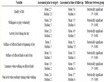
Table 1. SSTRA algorithm and estimated transfer function.
recursion bounds are identical as in Equation (9).
Now we can do something interesting. Consider a matrix result  with transfer function
  and another matrix result
  with transfer function
 , then we have

and more importantly small error increase.
The coefficient can be estimate as  but for simplicity here we set it
  (for ex-
ample  for one recursion
  for two and smaller and smaller).
So let us take again the Strassen algorithm and introduce a permutation instruction that allows us to switch on
Table 2. SW algorithm and estimated transfer function.
and off the orthogonal algorithm (Table 3) and see what could be a reasonable bound.
If we write the recurrence equation as we did in Equation (8), and we solve it to estimate the magnitude, then we should explicitly introduce coefficient . Because the bound is a function of the recursion level, we specify the coefficient as
  where
where  is the recursion level.
 (12)
(12)
For the Winograd’s variants such as SW and SWOPT the orthogonal transformation is a little more complicated:
 (13)
(13)
Once again, the permutations are logical only, there is no data movement.
Table 3. Orthogonal SSTRA algorithm and estimated transfer function.
In Section 2.1, we introduce an algorithm that actually applies all four possible direction. The regular, the two above, and the following:
 (14)
(14)
We call this algorithm  and we shall present a description in Section 8. Basically, we overlap the four error direction evenly Table 4.
Note. We applied these same permutations to Strassen and Winograd stability vectors in Section 2.1 to lower the coefficient , which represents the error of the algorithms in Equation (2). These are optimizations that improve the accuracy of the algorithms using two different measures. The Transfer function is more empirical because it is determined by experimentation and it should provide tighter bounds (e.g., SWOPT algorithm for
Table 4. SW-4Permute Algorithm and Estimated transfer function.
matrix input [0, 1]).
How will it work in practice? In short, the orthogonal algorithm actually improves the transfer function in a significant way that will improve the maximum error as well. In the following, we shall summarize the error in Figures 8, 9, 10, 11 and 12.
We can see that the error direction changed dramatically and the transfer functions of Fast algorithm is getting closer to the regular MM. From the simple theory we developed, we understand that we cannot achieve a truly uniform distribution by using orthogonal algorithm transformation. What we can do is to attenuate the effects of the recursive narrow error into a specific location so as to avoid the overlap of large errors close to the same geographical location.
A curiosity: the SWOPT orthogonal algorithm has a heat spot clearly defined on the right side of the matrix result. Such a biased error may suggest that part of the matrix is small and it could be computed separately: for 5
recursions, we may have to recompute a very small matrix  and shave the error by about 10% - 20%. In
case the reader is wondering about any relation with the permutations introduced in [21] , those permutations do

Figure 8. Parameters: n = 42, n0 = 20, range = [−1, 1], and iterations = 10,000 (Left) Transfer Function and maximum σ2 (Right) Maximum Error histogram and maximum (maximum) error.

Figure 9. (Left) n = 21, n0 = 20, range = [−1, 1], one recursion, and iterations = 10,000 (Right) n = 86, n0 = 20, range = [−1, 1], three recursions, and iterations = 10,000.
not change the error direction and thus the error; we tested them and not reported here.
7. Error Practice
In this section, we will wrap up the experimental results by showing the properties of fast algorithms using relatively small matrix sizes. The goal is to compare what we can predict using transfer function versus maximum error.
We present different views of the error and we start by showing the maximum error and maximum transfer function, here we may use the term heat to indicate the transfer function for short.
In Table 5, we present the maximum heat, the maximum error and their ratio for matrices in the range [0, 1]. In Table 6, we present the results for the range [?1, 1]. We run 10,000 iterations to compute the maximum error and maximum heat.
For every algorithm and matrix range, the heat and maximum error are consistent measures of each other and in particular we show that the orthogonal permutation always improves both. We present also the ratio between maximum error and maximum heat to provide the multiplicative factor to . We notice that the factor has a range in between 4 - 10. A value of 4, means that the error is closer to normal distribution. Once again, we see that GSGEMM has smaller error and heat for the range [?1, 1]. As a rule of thumb, the max error and heat is two times smaller than for the matrices in the range [0, 1]. In combination with large multiplicative factor of 10, it seems that GSGEMM distribution for the range [?1, 1] has fat tails suggesting not a normal distribution.
We can appreciate quantitatively that permutation algorithms reduce the heat and the maximum error by half.
Maximum Heat vs. Maximum Error Location.
There is a correlation between the values of the maximum error and the maximum heat. The correlation is used to show that we can design better algorithms. Here, we address the geographical correlation: we show that the transfer function maps the most likely locations for the error.
In Figures 13 and 14, we present the heat map for the maximum error for all algorithms for matrices of size  and with positive and mixed range. The FastMM algorithms apply 4 recursions; for example, the Strassen algorithm has a cluster of
  error diagonal matrices. In practice, for each 10,000 iteration, we store and plot the location and the value of the maximum error. It is clear that the transfer function predicts the location of the maximum error. We can also appreciate better the ability of the orthogonal algorithms of spreading the maximum error. The distribution of the error is not as random as for the GSGEMM algorithm but closer to it.
The goal of the orthogonal permutation is to change the pattern of the error in sub computations in such a way to avoid their maximum contribution. As result, we are spreading the error across the result matrix. Differently, we can guide the distribution of the error accordingly to target any part or the result matrix; this could be inva-

Figure 10. (Left) n = 175, n0 = 20, range = [−1, 1], 4 recursions, and iterations = 10,000 (Right) n = 350, n0 = 20, range = [−1, 1], 5 recursions, and iterations = 10,000.
Table 5. Range [0, 1], maximum error, maximum heat, max/heat ~ 4.
Table 6. Range [−1, 1], maximum error, maximum heat, max/heat ~ 4.

Figure 11. (Left) n = 21, n0 = 20, range = [0, 1], two recursions, and iterations = 10,000 (Right) n = 86, n0 = 20, range = [0, 1], three recursions, and iterations = 10,000.

Figure 12. (Left) n = 175, n0 = 20, range = [0, 1], 4 recursions, and iterations = 10,000 (Right) n = 350, n0 = 20, range = 0, 1], 5 recursions, and iterations = 10,000.
luable in the case we know where to have the maximum accuracy. This tailoring of the algorithm to a result accuracy goal is novel and powerful; in contrast, this is not possible using regular matrix multiplications because of their uniformly distributed error.
Brent’s Connection.
Now we show that the error is function of the algorithm. Let us start by using Equation (2), which we present here again.
 (15)
(15)
In Figure 15, we present the estimate of the factor  of the equation. Here, we use
  instead of
  to emphasize that
  is the measured value of
  in previous equations and their values are different. In this case, we measure the maximum error
 . We measure the maximum error of the leaf
 . We divide the left
hand side of Equation (15) by , thus we have
 . We estimate that
  is linear in
  and thus we

Figure 13. Orthogonal FastMMW (Left) n = 175, n0 = 20, range = [0, 1], 4 recursions, and iterations = 10,000 (Right) n = 175, n0 = 20, range = [−1, 1], 4 recursions, and iterations = 10,000.

Figure 14. (Left) n = 175, n0 = 20, range = [0, 1], 4 recursions, and iterations = 10,000 (Right) n = 175, n0 = 20, range = [−1, 1], 4 recursions, and iterations = 10,000.
divide the LHS by . The linear relation is adequate because the leaf computation is based on a
  algorithm that satisfies such a property. Thus, we estimate
  from the equation:
 (16)
(16)
For comparison purpose, we show also the  in case we use the GSGEMM, showing the minimum bound
  and remember that the current bounds for Strassen and Winograd call for
  and
and , respectively. Stating the obvious first, this bounds says that large
  is bad and small
  is good.
As a function of the range of the input we have different factors. For the range [?1, 1] we have clear factors:  for Winograd’s variants and
  for Strassen. Also we notice that the orthogonal algorithms by permutations provide consistently better
  s, being more accurate. For positive matrices in the range [0, 1], we see clearly that SW algorithm is accurate as GSGEMM for small number of recursions. Three recursions provide a sweet spot, any larger and we can notice a difference in accuracy of the algorithm.
So we can see even if we use the standard way to measure the error and the standard bounds: we reproduce correctly what we already know about the algorithm and we show that orthogonal permutation affects the maximum error.
In Figure 16, we show the different estimation of  using the maximum of the transfer function (instead of the maximum error). In practice, the maximum is about
 , so quite on the right of the estimate by transfer function. The advantage of using the transfer function is a clear picture where the resolution of the orthogonal permutation and the different algorithms is quite clear. Notice that both methods order the algorithm consistently.
Recursion Connection.
In this work, we introduce the transfer function to estimate the recursive effect on the error, so that to create a different recurrence equation to solve. Our goal was to achieve a simplified bound such as in Equation (17)

Figure 15. Computation of the multiplicative factor  (Left) maximum error, range = [−1, 1], and iterations = 10,000 (Right) maximum error, range = [0, 1], and iterations = 10,000. On the ordinate, we present X, we recall that the
  is the multiplicative factor, and on the abscissa we present N.

Figure 16. Computation of the multiplicative factor  (Left) maximum transfer function, range = [−1, 1], and iterations = 10,000 (Right) maximum transfer function, range = [0, 1], and iterations = 10,000.
 (17)
(17)
Even simpler using  as before
 (18)
(18)
The bound in Equation (18) is simpler to explain to any developer because we quantify the intuitive idea that more recursive calls will increase the error: the multiplicative factor is specific to the algorithm and a constant at each recursion step.
Both equations provide a means for the comparison of different algorithms and their accuracy. We can actually plug in the GSGEMM, which should provide a practical and theoretical lower bounds (X = 2).
In Figure 17, we estimate the factor  of Equation (2) using the maximum of the transfer function. In Figure 18, we present the analogous estimation using the maximum error. Let us start with the obvious:
  tries to explain the multiplicative factor of the leaf error so that to estimate the error of the algorithms. We present again GSGEMM to provide a lower bound.

Figure 17. Computation of the multiplicative factor X (Left) maximum transfer function, range = [−1, 1], and iterations = 10,000 (Right) maximum transfer function, range = [0, 1], and iterations = 10,000, We report X on the ordinate, we recall that  is multiplicative where
 , we present N = n problem size on the abscissa.

Figure 18. Computation of the multiplicative factor X (Left) maximum error, range = [−1, 1], and iterations = 10,000 (Right) maximum error, range = [0, 1], and iterations = 10,000.
We notice that the transfer function and the maximum error provide very similar estimate of . The order of accuracy is consistent. We see once again that for positive matrices SW should not have more than three recursions.
The recurrence solutions presented in Equations (9), (12), (19), and (20) are consistent estimate of the bounds; that is, they allow comparing the algorithm accuracy. However, they seem overestimating the measured ones.
8. Conclusions
In summary, from the theory of weak stability we introduce the family of orthogonal algorithms for the Fast- MMW algorithms. The combination of the regular and orthogonal algorithms allows us to write more accurate FastMMW algorithms. We show this theoretically by showing better error bounds. We provide extension to the error bounds, and the way we can compute error bounds, so that we can model corner cases: we introduce the transfer function. In fact, for the family of random matrices the weak stability bounds cannot capture idiosyncrasies when positive random matrices are used as operands.
Recalling conversations we had about error analysis, now we understand better why Winograd’s algorithms are viewed with suspicion by some even for positive matrices. In contrast, we have always found our Winograd implementation quite accurate for positive matrices. The misunderstanding is related to the assumption that all fast algorithms have the same error analysis properties. In this work, we show that we can actually estimate and expect accuracy: this is a property of the algorithms, their implementation, and the way we use them. Hopefully, a better understanding of these algorithms will provide adequate standard and error estimate in such a way to guide experiments and data collection: so as to make sense of large errors in experiments results (e.g., [22] ) sometimes due to other external factors and not algorithmic dependent.
We have the opportunity to open a new chapter and create new interest in this beautiful field.
Acknowledgements
This work stems from a question raised during a conversation with Matthew Badin, Alexandru Nicolau, and Michael Dillencourt. The question was: where the error is located? Once we answered the question by the transfer function, we wanted to reduce the error by randomizing the error pattern in particular by permutations. Marco Bodrato had the idea of permuting the computation among recursion calls. We revisited the permutation used by David Wise and checked the original use of the permutations. Wise’s permutations did not help because they are symmetric and they just reverse the order of the computation. Random permutations involving the result matrix did change it by disrupting the patter. The randomization and the permutations provided almost the same distribution as the original matrix multiplication: Richard Brent guided us to make sense of the preliminary result. At this stage, we had a randomized algorithm. This helped a little the maximum error. So instead of applying random permutations, we tried to understand which computation and permutation we could use systematically. The orthogonal permutations were crystallized and applied to random matrices: we achieved better transfer function and better error. Nicholas Higham asked whether or not this approach can be extended to general matrices and thus provide better bounds. The answer was yes, thanks to the theory developed by Dario Bini and Grazia Lotti in their original work. Orthogonal algorithms are applied to the stability vectors and thus reducing the asymptotic stability factor. We shared the preliminary draft of this work with all of the above and we thank them to be our sounding board, our reference, and our standard. Especially, we thank Richard Brent for his feed- back, moral support and clean up of the earlier drafts.
References
- Strassen, V. (1969) Gaussian Elimination Is Not Optimal. Numerische Mathematik, 14, 354-356. http://dx.doi.org/10.1007/BF02165411
- Douglas, C.C., Heroux, M., Slishman, G. and Smith, R.M. (1994) GEMMW: A Portable Level 3 BLAS Winograd Va- riant of Strassen’s Matrix-Matrix Multiply Algorithm. Journal of Computational Physics, 110, 1-10. http://dx.doi.org/10.1006/jcph.1994.1001
- Demmel, J. and Higham, N. (1992) Stability of Block Algorithms with Fast Level-3 BLAS. ACM Transactions on Mathematical Software, 18, 274-291. http://dx.doi.org/10.1145/131766.131769
- Demmel, J., Dumitriu, J., Holtz, O. and Kleinberg, R. (2006) Fast Matrix Multiplication Is Stable.
- Brent, R.P. (1970) Error Analysis of Algorithms for Matrix Multiplication and Triangular Decomposition Using Wi- nograd’s Identity. Numerische Mathematik, 16, 145-156. http://dx.doi.org/10.1007/BF02308867
- Miller, W. (1975) Computational Complexity and Numerical Stability. SIAM Journal on Computing, 4, 97-107. http://dx.doi.org/10.1137/0204009
- Bini, D. and Lotti, G. (1980) Stability of Fast Algorithms for Matrix Multiplication. Numerische Mathematik, 36, 63- 72. http://dx.doi.org/10.1007/BF01395989
- Edelman, A. and Rao, N. (2005) Random Matrix Theory. Acta Numerica, 14, 233-297. http://dx.doi.org/10.1017/S0962492904000236
- Kolmogorov, A.N. and Uspenskiiq, V.A. (1987) Algorithms and Randomness. Theory of Probability and Its Applica- tions, 32, 389-412. http://dx.doi.org/10.1137/1132060
- Winograd, S. (1968) A New Algorithm for Inner Product. IEEE Transactions on Computers, 17, 693-694.
- Higham, N.J. (1990) Exploiting Fast Matrix Multiplication within the Level 3 BLAS. ACM Transactions on Mathe- matical Software, 16, 352-368. http://dx.doi.org/10.1145/98267.98290
- Higham, N.J. (2002) Accuracy and Stability of Numerical Algorithms. 2nd Edition, SIAM, Philadelphia. http://dx.doi.org/10.1137/1.9780898718027
- Badin, M., D’Alberto, P., Bic, L., Dillencourt, M. and Nicolau, A. (2011) Improving the Accuracy of High Perfor- mance Blas Implementations Using Adaptive Blocked Algorithms. In Proceedings of the 2011 23rd International Symposium on Computer Architecture and High Performance Computing, SBAC-PAD ’11, Washington, DC, IEEE Computer Society, 26-29 October 2011, 120-127.
- Castaldo, A.M., Clint Whaley, R. and Chronopoulos, A.T. (2008) Reducing Floating Point Error in Dot Product Using the Superblock Family of Algorithms. SIAM Journal on Scientific Computing, 31, 1156-1174. http://dx.doi.org/10.1137/070679946
- Dongarra, J.J., Du Croz, J., Duff, I.S. and Hammarling, S. (1990) A Set of Level 3 Basic Linear Algebra Subprograms. ACM Transaction in Mathematical Software, 16, 1-17. http://dx.doi.org/10.1145/77626.79170
- Goto, K. and van de Geijn, R.A. (2008) Anatomy of Highperformance Matrix Multiplication. ACM Transactions on Mathematical Software. http://dx.doi.org/10.1145/1356052.1356053
- Priestley, M.B. (1981) Spectral Analysis and Time Series. Academic Press Inc, New York.
- Brockwell, P.J. and Davis, R.A. (2006) Time Series: Theory and Methods. Springer, New York.
- D’Alberto, P., Bodrato, M. and Nicolau, A. (2011) Exploiting Parallelism in Matrix-Computation Kernels for Symme- tric Multiprocessor Systems: Matrix-Multiplication and Matrix-Addition Algorithm Optimizations by Software Pipe- lining and Threads Allocation. ACM Transaction in Mathematical Software, 38, 1-2.
- Welch, P.D. (1969) A Fixed-Point Fast Fourier Transform Error Analysis. IEEE Transactions on Audio and Electroacous- tics, 17, 151-157. http://dx.doi.org/10.1109/TAU.1969.1162035
- Loos, S. and Wise, D.S. (2009) Strassen’s Matrix Multiplication Relabeled.
- Li, J.J., Ranka, S. and Sahni, S. (2011) Strassen’s Matrix Multiplication on Gpus. 2011 IEEE 17th International Conference on Parallel and Distributed Systems (ICPADS), Tainan, 7-9 December 2011, 157-164.
Appendix
SWOPT
If we take the expected transfer function from the experiments and estimate the transfer function, then we can explain the transfer function for matrices in the range [?1, 1] very nicely. If we take the minimum and the maximum of the transfer function we have a ratio as in Figure 1 of 4.
However, for matrices in the range [0, 1] and for the algorithm SWOP, the addition of the transfer function related to the matrix  does not explain the result Table 7. The transfer function estimation as above will fall short explaining experimental results.
The computation of  is based on the following set of operations executed left to right:


The computation of  has the right matrix operand that will be in the range [?1, 1] and thus with a smaller transfer function. There are two interesting features about the computation: the order of the additions such as
  is the same in
  and
and  and with higher probability to be positive. Also
  has higher probability to be positive implying that the errors are aligned so that the cancellation in
  and
and  are better than expected.
Table 7. SWOPT Algorithm and Estimated transfer function.
1The statistical properties of the error will not necessarily follow the statistical properties of the input matrices.
SW as accurate as SGEMM in theory.
Let us consider the algorithm deployed in SW and presented in Table 6 If we take the expected transfer function from the experiments and estimate the transfer function, then we can explain the transfer function for matrices in the range [?1, 1] very nicely. When we consider the other range [0, 1] and we observe that a few of the leaf computation are MM of mixed sign, we can estimate half of the contribution. The Fast MM for positive matrices is actually more accurate because the leave computations are not positive matrices.
The error we commit in the mixed-sign leaf MMs is smaller than for positive leaf MMs. There is a common knowledge that Winograd algorithm is more accurate because there is no true subtraction of the matrix products. Actually, the algorithm with only addition of the matrix result, will require subtraction in the input of the matrix product.
If we like to create a recursive equation to estimate the transfer functions:
 (20)
(20)
With a factor 2.5 and for small number of recursion, SW is very close to the regular MM. We can forecast and we show in practice that for , SW is as accurate as SGEMM and for
  we better switch algorithm. This is a proof for the consistent better accuracy for this particular variant Winograd algorithm for positive matrices.
SW-4PermuteL: four-permutation algorithm.
 (21)
(21)
NOTES

1The statistical properties of the error will not necessarily follow the statistical properties of the input matrices.