Natural Resources
Vol.4 No.1(2013), Article ID:28997,12 pages DOI:10.4236/nr.2013.41002
Modeling Resource Use Responses to Macroeconomic Changes: Water in the US Southern Great Plains*
![]()
Department of Agricultural and Applied Economics, Texas Tech University, Lubbock, USA.
Email: justinw@sorghumcheckoff.com, don.ethridge@ttu.edu
Received October 2nd, 2012; revised November 17th, 2012; accepted December 9th, 2012
Keywords: Macroeconomic Impacts; Ogallala Aquifer; Optimization; Recession
ABSTRACT
This study addressed the impacts of the 2008 US recession on water extraction rates from the Ogallala Aquifer in the Southern High Plains of Texas by examining the differences in projected macroeconomic variables and how they impact agricultural production and irrigation water use. The approach used preand post-recession FAPRI-based projections of commodity markets and an economic optimization model formulated for the Ogallala Aquifer to simulate water use adjustments. Results indicate that, based on the projections used, the 2008 recession decreased, then increased water use slightly in the representative counties, ceteris paribus, with minimal cumulative effect, and water use responsiveness to economic forces within the region was variable. This analysis also demonstrates that relating policy and economic changes to resource use changes is possible.
1. Introduction
Economic analyses of the impacts of changes in technologies, market shocks, and government policies and programs typically focus on surplus measures, prices, quantities, revenues and/or costs. While impacts on resource use may be implicit in these analyses through the derived demand for inputs, resource use impacts typically receive secondary, if any, attention. However, as concerns about resource sustainability grow, those resource impacts become more relevant to some public interests and policy makers.
Water is a key resource for both agriculture and the public at large. In 2008, 54.9 million acres of US cropland were irrigated, covering approximately 12% of all cropland [1], much of which occurred over the Great Plains in states such as Nebraska, Kansas, and Texas. On the Texas High Plains the southern portion of the Great Plains irrigated acres produced 60% of the states’ irrigated cotton and nearly 80% of the irrigated corn [2]. Throughout the southern and central Great Plains region, the Ogallala Aquifer (Figure 1) provides most of the
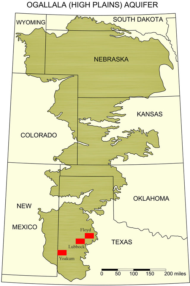
Figure 1. The Ogallala Aquifer, with location of study counties. Source: high plains underground water conservation district #1 [3].
groundwater needed for irrigation, accounting for nearly 65% of the irrigated acreage in the US [3]. However, since irrigation development began in the late 1940s, there has been a general persistent decline in available water from the aquifer from extraction rates exceeding recharge1. Understanding the water use implications of changes in technologies, economic phenomena, and policies is an important component of effective regional water use planning. The southern portion of the Ogallala, where the aquifer is generally the most accessible but most limited in quantity, was among the first to rapidly develop irrigation, and where depletion issues first became obvious. Consequently, the area tended to adopt water efficient irrigation application technology most rapidly. To date, regulatory limitations on pumping have not been implemented.
Theory and empirical studies have shown that commodity and input prices affect resource use, and policies, programs, changes in business cycles, recessions, or other factors may affect prices. Recent events have provided a natural experiment that may aid in understanding the linkages. Until 2007, the US had been through a relatively long period of economic growth with generally rising or relatively flat, although variable, agricultural commodity and energy input prices. In 2008, the start of a recession created uncertainty and altered future expectations within the agricultural market system.
This study addressed the impacts of the 2008 US recession, on water extraction from the Ogallala Aquifer in the Southern High Plains. The approach focused on representative water resource situations in the region and utilized preand post-recession FAPRI-based projections of commodity markets to simulate the adjustments in water use caused by changes in those macroeconomic variables. From a broader perspective, this analysis also serves to empirically demonstrate how external forces may work through economic incentives to impact resource use.
Macroeconomic forces (economic growth, interest rates, exchange rates, etc.) are known to impact individual sectors of the economy, including the agricultural sector. The direct effects on the agricultural sector are typically through variables such as commodity prices, exchange rates, interest rates, and production input costs. Resulting shifts in production of agricultural commodities, in turn, spill back to affect aggregate output, prices, other markets, and trade balances. Prior studies of the macroeconomic impacts in agriculture have focused on either structural changes that could occur within the dynamics of the economic system or broad characteristics within the market such as land values, consumer expendituresand agricultural incomes [4-6]. This study adds to the existing literature by focusing attention on the implications of macroeconomic changes on resource use. At the same time, the paper provides a framework for relating resource use to the broader market for future policy analysis.
2. Conceptual Framework
The basic model of groundwater irrigators’ profit is based on economic, hydrologic, and agronomic factors [7]:
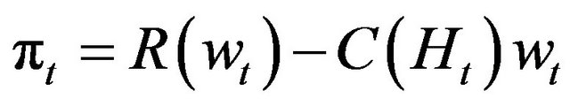 (1)
(1)
where πt = profit in time period t, R(w) = net farm revenue from water use, except for pumping costs (which depends on crops produced, crop yield functions, commodity values, and crop costs of production of all factors except water pumped), and C(H) = cost per acre of pumping water, which varies with pumping lift (that varies over time based on aquifer flow factors, aquifer volume, and aquifer yield of water.
The Ogallala is an unconfined underground aquifer (an impervious clay-lined bottom with the layers of soil over it not sealed), consisting of water deposited several million years in the past in a layer of water-bearing sand. The strata lies at different depths below the surface, varies in its thickness, and the sands yield water at different rates, all of which impact cost of water pumped across the region. Environmental factors such as rainfall, temperatures, and soils, which also vary across the region, also affect agronomic and economic choices of crops grown and aquifer recharge rates from rainfall and percolation through the soil. Across the region, variable recharge rates have been small relative to water extraction, resulting in persistent aquifer depletion since the beginning of irrigation development in the late-1940s.
The complex decision for irrigators is how to optimize use of the depletable groundwater aquifer over time. From Equation (1) above, irrigators are assumed to attempt to maximize profit over the (variable) life of the groundwater resource. In the process, they determine rates of depletion of the aquifer. Factors that impact R and/or C in Equation (1) may affect the optimum profit and the rate of depletion of the aquifer. Thus, major variables affecting that decision include crop production possibilities, production functions, soil characteristics, rainfall levels and patterns, temperature levels and patterns (agronomic factors), water pumping lifts, well yields, water in storage, recharge rates (hydrologic variables that change as water is pumped), irrigation application technology, commodity values, and many different input costs (economic variables).
Irrigators make these decisions on the basis of these types of microeconomic variables, which are generated in a macroeconomic environment. Economic recessions consist of a slowing or decline in aggregate economic activity. As production in economic sectors declines, effects typically include rising unemployment, declining demand and prices in some goods markets, and declining demand and prices in some factors of production markets; these also typically recover once he economy recovers from the recession. Recession impacts on irrigated agriculture production and profit (and aquifer depletion rates) occur largely through the prices of commodities that agriculture produces and the prices of production inputs that agriculture uses. To the extent that commodity prices are reduced by a recession, commodity production and profit and inputs used may be reduced (differentially for different crops depending on the relative price reductions, nature of production functions, etc.). To the extent that input costs are reduced by a recession, input use, commodity production, and profits may be increased (differentially by inputs and commodities). The net outcome of such changes depend on the specific changes emanating from the particular recession and all of the relationships implicitly embodied in Equation (1) and the outcome becomes an empirical question.
3. Methods and Procedures
The approach used in this analysis was to 1) estimate the optimum combinations of irrigated crops and irrigation water use in three counties with different aquifer situations in the southern High Plains over a 10-year period based on the 2008 FAPRI 10-year projections of commodity prices and input costs [8], which were based on the available macroeconomic outlook in early 2008; 2) re-estimate the same situations using the 2009 FAPRI projections [9], which used the macroeconomic outlook after the recession was underway; and 3) analyze the projected irrigation water use differences, which represent the recession’s estimated impact on aquifer depletion. The analysis was conducted on a set of representative county situations rather than on the region as a whole because of the variation in irrigation conditions and water use patterns within the region. This facilitates understanding of resource use responses to the various underlying conditions but precludes empirical projections of aggregate water use for the region as a whole without estimating all individual situations and aggregating to the regional total.
The three counties selected were Floyd, Lubbock, and Yoakum counties in the southern High Plains region of Texas. These counties vary in climatic factors, hydrologic characteristics, soil types, and cropping patterns. Primary drivers of the crop mix allocations within each county are soil type and irrigation water availability. The general county level hydrologic characteristics and enterprise allocations are presented in Tables 1 and 2. Floyd County has more clay soils, produces more grain crops and less cotton (Table 1), and has the most irrigation water available, with the most saturated thickness and the highest well yields (Table 2). Lubbock County has a mixture of clay and sandy soils, is dominated by cotton, has the greatest amount of irrigated cotton (Table 1), and lies between the other two counties on irrigation water availability (Table 2). Yoakum County, with 39% of its major crop acreage under irrigation, has predominantly sandy soils, the lowest proportion of irrigated acreage in cotton and sorghum and the greatest in wheat, and is the only county in the study producing irrigated peanuts. Its water is the most limited, as evidenced by the least aquifer saturated thickness and lowest well yields, but the shallowest (and least costly) pumping lift (Table 2).
Table 1. Average county level crop patterns of major crops (2005-2009).

Source: National Agricultural Statistics Service [2].
Table 2. County level aquifer hydrologic characteristics (2009).
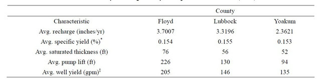
*Specific Yield is defined as the percentage of one foot of saturated sands in the Ogallala Aquifer that contain water; ‡Gallons per minute (GPM) based on Saturated Thickness (ST); GPM = 2.234*ST + 0.0078336*ST2 − 0.000282*ST3, [25].
3.1. The Model
Optimum crop combinations and water use were estimated using a non-linear dynamic economic optimization model that embodies hydrologic conditions, crop acreages, cost and revenue relationships, and crop yield functions for each county within the region. The framework, originally developed by Feng and Segarra [10] and later modified [11-17], is referred to as the Ogallala Model (OM). The model was estimated using the General Algebraic Modeling System (GAMS), a computer optimization program [18].
The objective function for each county is:
 (2)
(2)
where NPV is the net present value of net returns ($/acre); r is the discount rate; Ω is the expected average rate of yield increase through time (assumed to be 0 in this analysis); and NRt is net revenue at time t ($/acre). NRt is defined as:
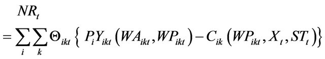 (3)
(3)
where i represents crops grown; k represents irrigation application system used [surface row irrigation; lowenergy, precision application sprinkler irrigation (LEPA); or sub-surface drip irrigation]; Θikt is the percentage of crop i produced using irrigation technology k in time t; Pi [s the output price of crop (in $/unit of crop produced); WAikt and WPikt is acre inches of irrigation water applied and water pumped, respectively; Yikt[∙] is the per acre yield production function for crop i, irrigation system k, and time t; Cikt ivariable production costs ($/acre) for crop i, irrigation system k, and time t; Xt is pumping lift (ft.) at time t; and STt is the saturated thickness of the aquifer (ft.) at time t.
The model constraints are:
 (4)
(4)
 (5)
(5)
 (6)
(6)
 (7)
(7)
 (8)
(8)
 (9)
(9)
 (10)
(10)
 (11)
(11)
 (12)
(12)
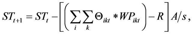
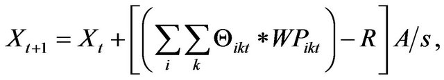
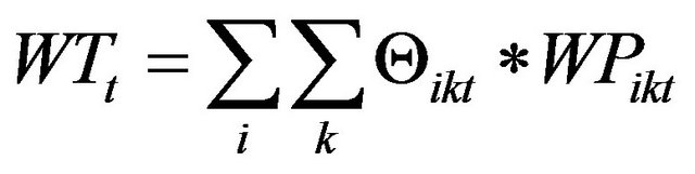
Equations (4) and (5) are equations of motion that update the two state variables, saturated thickness (STt) and pumping lift (Xt), where R is the annual recharge rate (ft.), A is the proportion of irrigated acres (initial number of irrigated acres in the county divided by the total area of the county overlying the aquifer), and s is the specific yield of the aquifer (percent of the saturated sand area in the aquifer that is water). Equations (6)-(8) are the water application and water pumping capacity constraints. GPC is gross pumping capacity (gpm), IST is the initial saturated thickness of the aquifer (ft.), and WY is the average initial well yield for the county (gpm). Equation (7) specifies the total amount of water that can be pumped per acre in time t, WTt, shows the sum of water pumped on each crop, and (8) requires WTt to be less than or equal to GPCt.
Equations (9) and (10) are the cost functions in the model. PCikt is the cost of pumping ($/acre) for crop i, irrigation technology k, in year t, EF is the electrical energy used for pumping (kwh), EP is the price of energy ($/kwh), EFF represents pump efficiency2, and 2.31 is a constant representing the height of a column of water, in feet, that will exert a pressure of 1 pound per square inch. Equation (10) expresses the cost of production, Cikt in terms of VCik. the variable cost of production ($/acre), HCikt, the harvest cost ($/acre), MCk, the irrigation system maintenance cost ($/acre), DPk, the per acre depreciation of the irrigation system ($/year), and LCk, the cost of labor ($/acre) for the irrigation system. Equation (11) limits the sum of an acre of all crops i produced by irrigation systems k for time period t to be ≤1. Equation (12) assures that all decision variables in the model take on non-negative values.
While the previous equations show the foundation for the optimization model, other constraints, scalars, and estimation procedures within the model provide a degree of stability for the solution through time. In this analysis, a key constraint was that crop acreage changes were limited to 2% per year. This constraint (1) ensured that the model did not rapidly shift acreage into high value crops that are not feasible on a regional scale and (2) is consistent with historical shifts of acreages within counties in the region. All irrigation was assumed to be with LEPA systems, the predominant irrigation technology used on the southern High Plains3. Technology advancements through crop genetics or conversions to more efficient irrigation technologies were not considered over the 10- year horizon of this analysis, but advancements are important for long-term (30 - 60 years) projections [20,21].
The component that makes the optimization model non-linear is the use of quadratic production functions. CropMan, a software program that estimates crop yields based on regional conditions such as rainfall, temperatures, and soils [22], was used to simulate county-specific crop yield-irrigation application estimates4. These were then used to estimate quadratic yield-irrigation water production functions using Ordinary Least Squares regression, and the production functions provided the adjustments in the optimization model for variations in irrigation water applications.
Given the 10-year price projections derived from the FAPRI baselines, the initial crop acreages5 and hydrologic conditions for the three counties, the optimization model was used to derive the net revenue maximizing crop production combinations and water use associated with them over the 10-year (2010-2019) period. Average climate conditions for each of the 10 years were assumed in both the FAPRI and OM projections. These solutions provided the basis for deriving 10-year projected cropping patterns and water use patterns under average hydrologic conditions for each of the three counties under the 2008 baseline projections (pre-recession), and under the 2009 baseline projections (recession). Comparison of these two solutions provided an estimate of the impact of the recession on irrigation water use in the three counties and a comparison across counties.
The 2008 and 2009 FAPRI projections showed variations in two primary variables that affect the irrigated production system and resource use-commodity prices and energy costs. The comparison described above captures only the combined effects of these, so two separate scenarios were evaluated for each of the FAPRI baseline projections to isolate the impacts of the shift in crop prices from the effects of energy costs. The first scenario was for the combined effect, described above. The second scenario held energy (production) costs at the 2008 levels and used price projections from the 2009 baseline. Thus, the comparison of the two baselines under scenarios one and two provided and estimate of the water use changes driven by the crop price changes alone and, by implication, changes driven by the shift in energy costs.
3.2. Data
The initial county level enterprise allocations and hydrologic characteristics are shown in Tables 1 and 2. Land devoted to other crops, along with the aquifer underlying that land, was omitted from the model; this effectively assumed that acreages in those crops and the water allocated to them did not change over the 10-year study period. Note that in Table 2 the parameters in the first two rows, recharge and specific yield, are constant over time in the model while parameters in the last three rows change over time as water is pumped from the aquifer.
The data used to categorize the irrigation components and aquifer characteristics were obtained from the Texas Water Development Board [23], the High Plains Underground Water Conservation District No. 1 [3], and the Texas Tech Center for Geospatial Technology [24]. All pumping plants were assumed to be electric submersible (the predominant type) and pumping cost was estimated based on brake horsepower requirements for the county average pumping depth, typical operating pressure, and the average pumping efficiency (60%). Initial well yields for each saturated thickness level were estimated using an equation developed by Lacewell et al. [25] and estimated values for recharge were based on work originally developed by Stovall [26].
Major macroeconomic and price projections from FAPRI [8,9] that impact this analysis are summarized in Tables 3 and 4. The world and US GDP growth projections indicate an economic slowdown in 2009 and 2010
Table 3. Sample of macroeconomic projections within the FAPRI 2008 and 2009 baselines.

*In local currency per US dollar.
Table 4. FAPRI projected prices* for the 2008 and 2009 baselines.
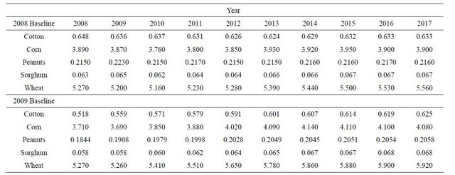
*Cotton ($/lb lint), Corn ($/bu), Peanuts ($/lb), Sorghum ($/lb), Wheat ($/bu).
from the recession with recovery thereafter. Exchange rate changes differed across countries in response to the differences in recession impacts on economies. Petroleum price projections showed a sharp decline in 2009 and 2010 from the recession, then recovery to higher prices in later years. Crop commodity price projections (Table 4) in the 2008 baseline showed a general increase, with the 2009 baseline projections having generally lower initial prices and different rates of growth during recovery; commodity markets are impacted differently by macroeconomic forces.
The FAPRI commodity price projections were localized by calculating the basis (average 1990-2007) between the national FAPRI prices and Texas prices [2] and applying that basis to the projections. Prices used in the analysis are shown in Table 5. Cotton prices include a weighted value for lint and cottonseed based on a 1:1.3 turnout ratio of lint to cottonseed.
Initial enterprise production costs for the three counties were obtained from Texas crop and livestock budgets [27], with costs and revenues in the enterprise budgets adjusted for each year of the ten year time horizon. Revenue adjustments used the price projections shown in Table 5; yield changes from technology were assumed to be 0 over the period of the study due to the uncertainty of that technology but yields were allowed to vary with irrigation water application rates through the production functions embodied in the model. Cost adjustments on electricity and labor were based on FAPRI projections of those items Excluding electricity and labor costs, all other cash field expenses were shifted based on the changes in US indices of prices paid by farmers provided by the FAPRI outlook (Table 6). FAPRI projections had the primary differences in production costs due to fuel (energy); fuel costs declined more rapidly with the recession but recovered over time. Farm program income such as direct and counter-cyclical payments or crop insurance programs were not included within the revenue calculations of this analysis because they have little, if any, effect on crop selection decisions. The initial electricity rate to pump irrigation water in the region was from the Texas Utilities Commission for the Southwestern Public Service Pool. This rate ($14/kwh) was adjusted for each year of the planning horizon using FAPRI’s projections of percentage changes in cost of fuels.
4. Results
Results are presented by county and scenario. The first sub-section explains the estimated overall effects of the recession on irrigation water use over the 10-year horizon and the second explains the estimated impacts of commodity price and production (energy) cost shifts associated with the recession and compares the scenario results.
4.1. Scenario 1—Projections with Price and Energy Cost Changes
Projected optimal crop acreages under the 2008 baseline are shown in Table 7; 2008 acreages changed from the historical patterns (Table 1), but not by large magnitudes. Projected irrigated acreages of all crops in each county decreased over time, as expected. Crop mixes remained largely unchanged, but total production of all crops decreased. Water use projections (Table 8) showed differences in the amounts of water pumped across counties. Floyd County, with relatively more water available to pump (higher saturated thickness of the aquifer), increased pumping from the aquifer over the 10-year period, with a cumulative increase of 3.15% over ten years. This change was possible because there was sufficient capacity for increased pumping to occur. Floyd County was projected to decrease pumping during the recession, but increased pumping as recovery occurred. In this case, a decline in the price of electricity caused the water use to increase slightly, which increased yields, which compensated for the 2009 decrease in commodity prices. Similar adjustments would likely occur in counties that have relatively high water available to irrigate and are not at maximum pumping capacities.
Table 5. Localized projected prices* for the 2008 and 2009 baselines.
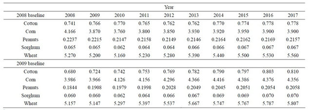
*Cotton ($/lb lint), Corn ($/bu), Peanuts ($/lb), Sorghum ($/lb), Wheat ($/bu).
Table 6. FAPRI projected annual percentage changes in costs of production items; 2008 and 2009 baselines.
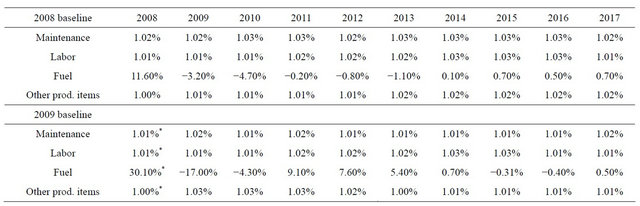
*Actual.
Table 7. Projected crop acreages from 2008 baseline, by county.
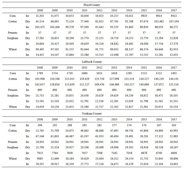
Table 8. Water use by county and year, scenario 1.
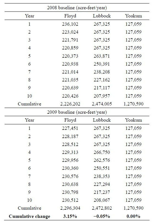
Lubbock and Yoakum counties exhibited different reactions to the recession relative to Floyd County. These counties had little or no cumulative changes in irrigated crop water use. Cumulative water consumption in Lubbock dropped slightly (−0.05%), while Yoakum showed no change. Lubbock and Yoakum counties lack the capacity to increase pumping. Lubbock County was projected to have a small decrease in pumping, then increased pumping with economic recovery; Yoakum County was projected to have no variation in irrigation withdrawals.
Thus, the model results for scenario 1 indicate that the overall estimated impact of the recession increased cumulative water withdrawals from the Ogallala by a relatively small amount, but not uniformly across the region and with different withdrawal patterns through time. Cumulative water withdrawals increased when aquifer conditions provided sufficient water to permit increased pumping. Also, where groundwater is relatively more abundant, the more likely farmers were to decrease water use in response to the recession, then increase water use later during economic recovery (and cumulatively use more water over the 10-year period). Thus, under the conditions projected in the FAPRI projections for this particular recession and the assumptions underlying the OM structure, scenario 1 results indicate that the increased incentive to use more water due to lower pumping costs associated with the lowered energy costs from the recession outweighed the incentive to use less water due to lower commodity prices from the recession when producers had remaining pumping capacity. In cases where producers were already at their pumping capacity, the recession had no impact on water use, but there was an impact on net returns.
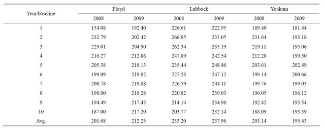
With commodity prices, input costs, production, and water use all changing, effects on projected net returns from scenario 1 are shown in Table 9. The projected pattern was for the collective recessionary impacts to decrease farm income, but with the decrease diminishing with economic recovery, and cumulative negative impacts on farm income over the 10-year period.
4.2. Scenario 2—Projections with Energy Costs Constant and Comparisons
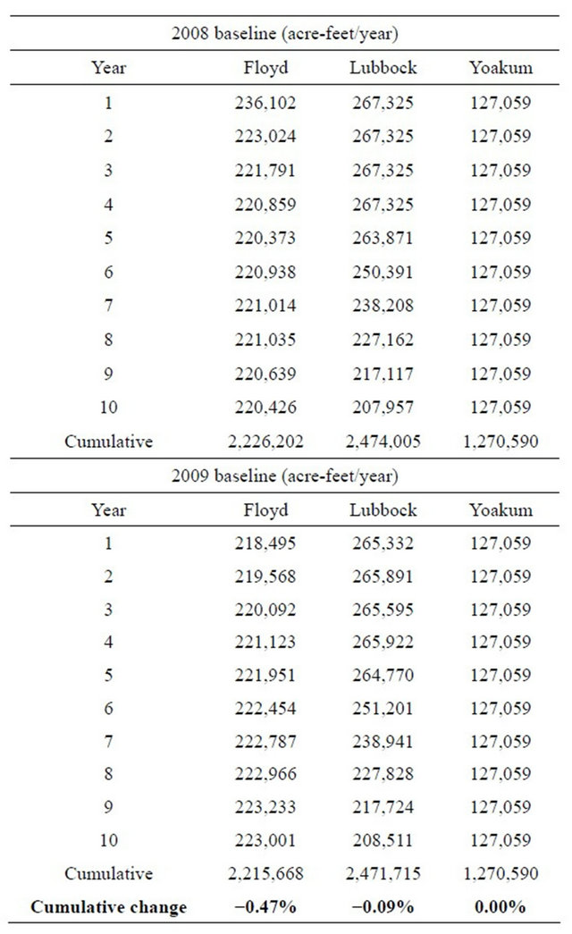
Crop acreages in scenario 2 did not change from scenario 1 (Table 7 also shows crop acreages for scenario 2), although farm income fell relative to the 2008 baseline (Table 10). However, with production costs held at 2008 baseline projections, net revenues were higher under scenario 2 (the projected effect of the recession on farm income was less from the commodity price changes than from the production, largely energy, cost changes). The scenario 2 ten year water use projection results are shown in Table 11. In this scenario, Floyd County had a slight cumulative water use decline (−0.47%) instead of the slight increase (3.15%) under scenario 1. Lubbock County showed a 0.09% decrease compared to the 0.05% decrease in scenario 1and Yoakum County had no change (0.00%) in both scenarios.
Comparison of the time patterns of water use in Table 10 show that, as in scenario 1, both Floyd and Lubbock counties decreased water use in response to the recession commodity price declines, and by a larger decline than in scenario 1 (Table 8), then increased water use with economic recovery, but by a smaller increase than in scenario 1 (the input cost decline did not occur with scenario 2). Yoakum County showed no water use response to the recession in scenario 2, as in scenario 1.
Thus, as commodity prices declined, ceteris paribus, producers in two out of the three counties responded to the projected recessionary impacts by lowering water use, then increased water use in recovery, with a slight cumulative decrease over the 10-year period; this result is logical and not inconsistent with theoretical expectations. The lack of response in Yoakum County may be due to their water resources being committed to the point of no flexibility, at least within the range of price and cost
Table 9. Weighted returns over variable costs ($/acre), by year and county, scenario 1.

Table 10. Weighted returns over variable costs ($/acre), by year and county, scenario 2.
variations represented in this analysis. Generally, water use in these simulations became less responsive to the economic conditions analyzed as aquifer conditions approach exhaustion.
Comparing scenarios 1 and 2 also suggests that within the Southern High Plains and the groundwater situations represented in this analysis, water use is likely more responsive to variations in the cost of pumping water than to variations in commodity prices, at least within the range of changes caused by the 2008 recession. While in general (across the three counties represented in this study) the lowering of commodity prices represented by the recession caused a decline in water use and the lowering of input (energy) costs and caused an increase in water use. In this case, the latter effect was larger than the former. Comparisons across counties suggest that the nearer (farther) the water resource use is to capacity, the less (more) responsive water use is to shifting macroeconomic factors, commodity prices, and water pumping costs.
5. Summary and Conclusions
This study simulated the impacts of the 2008 recession on water use on the Southern Great Plains using two existing analytical modeling systems the FAPRI baseline projections for 2008 and 2009 (the differences representing the recession impacts) and an optimization model embodying aquifer hydrologic characteristics (“Ogallala Model”). The FAPRI projections were driven by the expected shifts in macroeconomic projections and translated them into commodity and input market projections that impact irrigation water use decisions at a farm and regional production level. The optimization model estimated the impacts of the projected commodity price and
Table 11. Water use by county and year, scenario 2.
input cost changes through time (a 10-year period) on crop production and irrigation water use in the southern portion of the Ogallala Aquifer. Three counties were analyzed, representing different crop mixes and aquifer characteristics. Because the recession initially led to decreased commodity and input cost decreases, which affect crop output and water use in opposite ways, two scenarios were run to isolate the impacts of commodity price changes from input price changes from the recession.
The results of this study show that in the southern portion of the Great Plains’ Ogallala Aquifer the 2008 recession the expected effect was an initial slowdown of aquifer depletion, but an increase in the depletion rate as the economy recovers such that the expected net longterm cumulative effect on the depletion rate is minimal. Further, the impacts are not expected to be evenly distributed across the region. In locations where withdrawals are at or near capacity, the anticipated cumulative adjustments in water use appear to be unresponsive to the changes driven by the 2008 recession, and possibly others. In locations where the aquifer is further from depletion where there is more flexibility in pumping water use would likely adjust more, with a decrease in withdrawals in response to the recession and an increase with recovery. More specifically, water use within the region would be expected to respond to economic forces in the 2008 recession, but only where increased pumping flexibility exists. Further, expected water use in the region is likely more responsive to pumping costs than to commodity prices associated with the 2008 recession and the expected crop mix appears relatively unresponsive to both.
The approach used here presents a means of examining expected outcomes of a recession, and perhaps of other types of anticipated macroeconomic and/or policy changes on production sectors and resource (in this case, water) use, as opposed to examining or quantifying what actually happened (after the fact). These types of approaches may become more important as focus on water scarcity becomes of more interest. That is, the public interest in the expected impacts of economic variables on water use may become as important as their expected impacts on production and incomes.
REFERENCES
- Census of Agriculture, “Farm and Ranch Irrigation Survey Fact Sheet,” 2008. http://www.agcensus.usda.gov/Publications/2007/Online_Highlights/Fact_Sheets/fris.pdf
- National Agricultural Statistics Service, “Quick Stats: Agricultural Statistics Data Base,” 2008. http://www.nass.usda.gov/QuickStats
- High Plains Underground Water District, “The Ogallala Aquifer,” 2009. http://www.hpwd.com/the_ogallala.asp
- J. Baek and W. W. Koo, “On the Dynamic Relationship between US Farm Income and Macroeconomic Variables,” Journal of Agricultural and Applied Economics, Vol. 41, No. 2, 2009, pp. 521-528.
- G. E. Schuh, “The Exchange Rate and US Agriculture,” American Journal of Agricultural Economics, Vol. 56, No. 1, 1974, pp. 1-13. doi:10.2307/1239342
- B. Gardner, “On the Power of Macroeconomic Linkages to Explain Events in US Agriculture,” American Journal of Agricultural Economics, Vol. 63, No. 5, 1981, pp. 871- 878. doi:10.2307/1241262
- P. Koundouri, “Current Issues in the Economics of Groundwater Resource Management,” Journal of Economic Surveys, Vol. 18, No. 5, 2004, pp. 703-740. doi:10.1111/j.1467-6419.2004.00234.x
- Food and Agricultural Policy Research Institute, “FAPRI 2008: US and World Agricultural Outlook,” FAPRI Staff Report 08-FSR 1, 2008.
- Food and Agricultural Policy Research Institute, “FAPRI 2009: US and World Agricultural Outlook,” FAPRI Staff Report 09-FSR 1, 2009.
- Y. Feng, “Forcasting the Use of Irrigation Systems with Transition Probabilities in Texas,” Texas Journal of Agriculture and Natural Resources, Vol. 5, 1992, pp. 59-66.
- T. S. Arabiyat, “Agricultural Sustainability in the Texas High Plains: The Role of Advanced Irrigation Technology and Biotechnology,” M.S. Thesis, Texas Tech University, Lubbock, 1998.
- B. Das, “Towards a Comprehensive Regional Water Policy Model for the Texas High Plains,” Ph.D. Dissertation, Texas Tech University, Lubbock, 2004.
- J. W. Johnson, “Regional Policy Alternatives in Response to Depletion of the Ogallala Aquifer,” Ph.D. Dissertation, Texas Tech University, Lubbock, 2003.
- B. Terrell, “Economic Impacts of the Depletion of the Ogallala Aquifer: An Application to the Texas High Plains,” M.S. Thesis, Texas Tech University, Lubbock, 1998.
- E. A. Wheeler, “Policy Alternatives for the Ogallala Aquifer: Economic and Hydrologic Implications,” M.S. Thesis, Texas Tech University, Lubbock, 2004.
- E. Wheeler, B. Golden, J. Johnson and J. Peterson, “Economic Efficiency of Short-Term versus Long-Term Water Rights Buyouts,” Journal of Agricultural and Applied Economics, Vol. 40, No. 2, 2008, pp. 493-501.
- J. A. Weinheimer, “Farm Level Financial Impacts of Water Policy on the Southern Ogallala Aquifer,” Ph.D. Dissertation, Texas Tech University, Lubbock, 2008.
- A. Brooke, D. Kendrick, A. Meerdus, R. Raman and R. E. Rosenthal, “GAMS: A User’s Guide,” GAMS Development Corporation, Washington DC, 1998.
- G. Fipps, “Calculating Horsepower Requirements and Sizing Irrigation Supply Pipelines,” Texas Agricultural Extension Service Technical Bulletin B-6011, 1995.
- J. W. Johnson, P. N. Johnson, B. Guerrero, J. Weinheimer, S. Amosson, L. Almas, B. Golden and E. Wheeler-Cook, “Groundwater Policy Research: Collaboration with Groundwater Conservation Districts in Texas,” Journal of Agricultural and Applied Economics, Vol. 43, No. 3, 2011, pp. 345-356.
- S. L. Amosson, L. Almas, B. Golden, B. Guerrero, J. Johnson, R. Taylor and E. Wheeler-Cook, “Economic Impacts of Selected Water Conservation Policies in the Ogallala Aquifer,” Kansas State University Agricultural Experiment Station and Cooperative Extension Service, Staff Paper No. 09-04, 2009.
- T. J. Gerik, W. L. Harman, J. R. Williams, L. Francis, J. Greiner, E. Steglich, M. G. Magre and A. Meinerdus, “Crop Production and Management Model (CropMan) Version 3.2,” Blackland Research Center, Temple, 2003.
- Texas Water Development Board, “Survey of Irrigation in Texas,” Report 347, 2001. http://www.twdb.state.tx.us/publications/reports/GroundWaterReports/GWReports/R347.pdf
- Texas Tech Center for Geospatial Technology, “Texas Ogallala Summary,” 2009. http://www.gis.ttu.edu/OgallalaAquiferMaps/Default.aspx
- R. D. Lacewell and J. C. Pearce, “Model to Evaluate Alternative Irrigation Systems with an Exhaustible Water Supply,” Southern Journal of Agricultural Economics, Vol. 5, No. 2, 1973, pp. 15-21.
- J. N. Stovall, “Groundwater Modeling for the Southern High Plains,” Ph.D. dissertation, Texas Tech University, Lubbock, 2001.
- Texas Agrilife Extension Budgets, “Extension Agricultural Economics,” 2009. http://agecoext.tamu.edu/resources/crop-livestock-budgets/by-district/district-2/2008.html
NOTES
*Authors acknowledge support from the Cotton Economics Research Institute, the Thornton Agricultural Finance Institute, the CASNR Water Center, and the Texas Alliance for Water Conservation Project, Texas Tech University, and the USDA through the Ogallala Aquifer Program (Project # 58-6209-9-05-054) and the Cotton Policy Analysis Project (#2010-38868-20846). Authors also thank Phillip Johnson, Jeff Johnson, and Chenggang Wang for their helpful reviews of prior versions of this manuscript.
1The rate of decline varies across well sites from variations in pumping rates, well spacing, aquifer hydrologic characteristics, and recharge rates. Recharge rates vary with rainfall and soil percolation rates [3].
2Pumping plant efficiency is a combination of the efficiencies of the separate components of a pumping system (power unit, pumping drive or gear head, and pump), which impacts the cost of pumping an acre inch, In the case of centrifugal electric pumps, the maximum attainable efficiency is 75% - 82% [19] Pumping efficiency was assumed to be 60% in this study.
3Some surface row irrigation still exists and some sub-surface drip irrigation systems are in use, but data on acreages under these applications do not yet exist and they are known to be small in relation to acreage under LEPA.
4Comparisons of CropMan estimates and county data showed that the program performs well in estimating county average yields while normally underestimating yields based on the latest genetic advancements.
5Livestock (stocker cattle) grazing was also included in the model, but discussion of them is omitted here because they did not enter any of the solutions during the period of this analysis.