Open Journal of Biophysics
Vol.2 No.2(2012), Article ID:18919,8 pages DOI:10.4236/ojbiphy.2012.22005
Reproducing Cochlear Signals by a Minimal Electroacoustic Model
1Institute of Otolaryngology, School of Medicine, Catholic University, Rome, Italy
2Department of Information Engineering, Electronics and Telecommunications, Sapienza University, Rome, Italy
3Department of Environment and Primary Prevention, Istituto Superiore di Sanità (I.S.S.), Rome, Italy
4Department of SAIMLAL, Section of Anatomy, Sapienza University, Rome, Italy
Email: *colosimo@caspur.it
Received January 21, 2012; revised March 15, 2012; accepted March 22, 2012
Keywords: Otoacustic Emissions; Recurrence Quantification Analysis; Biosignals
ABSTRACT
Transient-Evoked Otoacoustic Emissions (TEOAEs) were studied, with particular reference to their subject-dependent features. To this end, an electric model of the ear was implemented and validated. Simulated and natural TEOAEs were analyzed through a nonlinear analysis technique. The simulated signals were able to reproduce the dynamical features of the experimentally observed TEOAEs and, most importantly, the natural variability among individuals. The unexpected inverse relation between model complexity and adherence to the natural signals is commented.
1. Introduction
Otoacoustic Emissions (OAEs) are low-level amplitude acoustic signals generated in the inner ear and measurable in the external auditory canal. Since their discovery [1] they have been extensively used in clinical applications thanks to their reproducibility and stability.
The Transient Evoked OAE (TEOAEs) considered in this paper are signals evoked by an external stimulus. They include a passive ringing linearly dependent on the incident stimulus and with short latency, followed by a smaller, nonlinear, long latency and long duration oscillation.
Natural TEOAEs have been successfully investigated [2,3] by means of Recurrence Quantification Analysis (RQA) and simulated on the basis of different models of the human hearing function [4]. A first group of models, such as the gammatone model [3,5] or the electronic cochlea [6], aims to reproduce the shape of TEOAEs with no specific consideration to the involved anatomical structures. Another group of models emphasizes the correspondence between ear anatomy and model elements. The ear model developed by [7,8], for example, relies on the electro-acoustic analogy [9] and provides clues to both speech and hearing research.
We implemented such a model and compared simulations and natural signals by means of RQA and Principal Components Analysis (PCA) in the aim to reproduce the natural variability of TEOAEs. Unexpectedly, a better match with natural signals was obtained by the less complicated model in terms of active cochlear modules. This is in line with the idea that reproducing complex biological phenomena, resulting from a manifold of nonlinear interactions, does not necessarily require complicated physical models [10]. This is also important since modeling the natural inter-individual variability is by far more relevant in biomedicine than the classical reproduction of ideal cases.
2. Methods
2.1. Recording and Simulating TEOAEs Signals
Natural TEOAEs responses were obtained in the Audiology Department of Palermo University, Italy, from 104 healthy subjects (50 males, 54 females; age: 27.7 ± 8.2 yr). The signals were recorded by the ILO88 system (Otodynamics) according to the protocol described in [2]. A schematic overview of the human ear and of the electronic model [7,8] is reported in Figure 1.
In the electro-acoustic analogy the outer ear is represented as a uniform transmission line [11], the middle ear as a complex electrical network [12] and the cochlea as a transmission line with a variable number of partitions able to simulate active processes. In particular, each partition contains a series inductor, a shunt resonant circuit and a non-linear voltage source. As for the parameters used in the simulations, see the table Appendix.

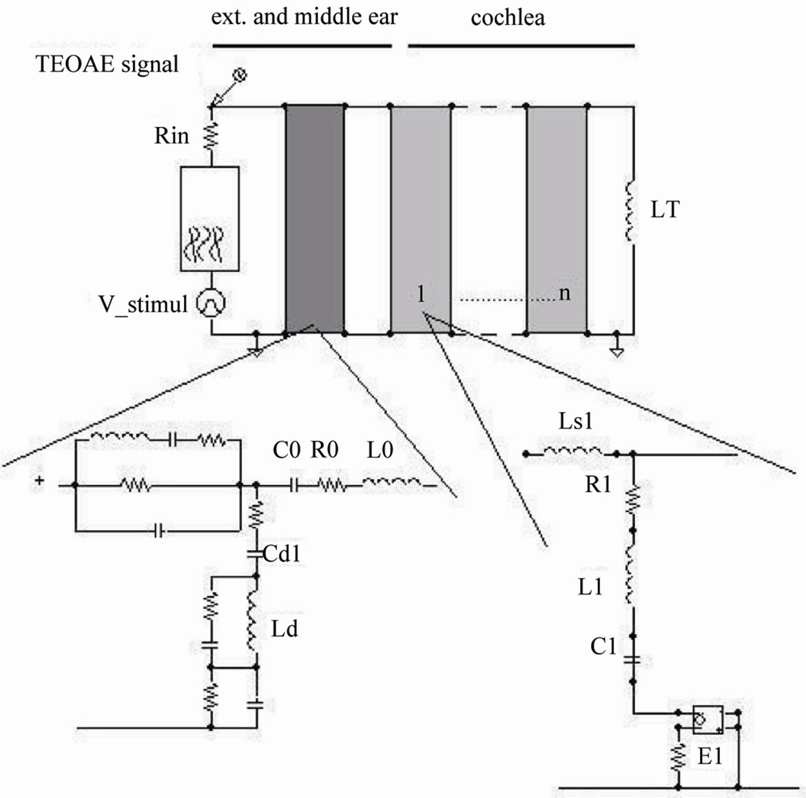
UP: The snail-like shape typical of the cochlea, is unwound to show the tonotopic features of its functional partitions, whose number is of the order of 3.5 × 10³ in the normal ear. Each partition acts as a resonator at a frequency (indicated) inversely proportional to its distance from the base. BELOW: An electric model of the ear including the auditory canal, the middle ear, and the cochlea (see the text for details).
Figure 1. Simplified view of the human ear and of the electronic model.
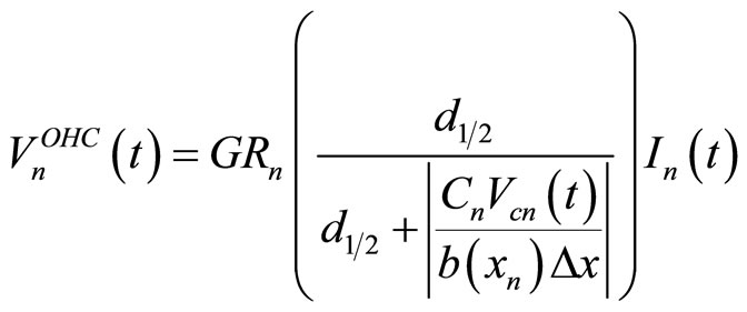
The model equations were solved using PSpiceTM, a standard electrical simulation tool previously used to study an entirely passive electric model of the cochlea [13]. The voltage source of the n-th cochlear partition used to simulate the OHC’s active processes can be defined [7] as:
 (1)
(1)
where  is a gain factor,
  ,
,  , and
, and  are the resistance, capacitance, and current of the n-th cochlear branch,
  is the voltage drop across
 ,
,  is a constant, and
 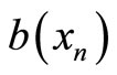 is the basilar membrane segment area represented by the n-th branch. Equation (1) has been reworked to make it suitable for implementation into PSpiceTM as:
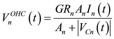 (2)
(2)
where:
 (3)
(3)
Equation (2) shows the dependence of OHC voltage sources on the ratio between the current in the cochlear branch and the voltage across . The input voltage is a rectangular pulse 80 µs wide corresponding to a stimulus of 80 dB SPL.
2.2. RQA-PCA of TEOAEs Signals
RQA is a technique used to quantify the amount of deterministic structure of short, non-stationary signals [14, 15] and to pick sudden phase changes possibly underlying mechanistically relevant phenomena.
The RQA descriptors of each signal can be worked out from the corresponding recurrence plot (RP). A RP is reckoned as follows:
• An embedding matrix (EM) is built, where the first column is the time series representing the signal and the following columns are time-lagged copies of it;
• A distance matrix is evaluated, whose  element is the Euclidean distance between the i, j rows of EM;
• If  is lower or equal to a predefined cut-off value (radius), the i, j location in the RP plot is darkened, marking a recurrent point, otherwise it is left blank.
RQA showed quite useful in the analysis of many physiological signals [16,17] as well as of spatial series like DNA and protein sequences [18]. A detailed discussion of such applications is in the seminal paper by Webber and Zbilut [15], while a complete review of the method can be found in [19]. On the basis of previous works [3,20], the RPs of our signals have been quantified using the following descriptors:
• % Recurrence, fraction of the plot occupied by recurrent points, measuring the amount of periodic and auto-similar behavior of the signal;
• % Determinism, fraction of recurrent points aligned parallel to the main diagonal, indicating the degree of deterministic structure due to the presence of quasiattractors [14].
• a Shannon entropy, estimated over the distribution of the length of deterministic lines, linked to the richness of deterministic structure.
Finally, a non redundant picture of the information provided by the RQA descriptors may be obtained by means of PCA, which allows to reduce the data set dimension without noticeable loss of information (see Appendix).
Using a set of 70 TEOAEs signals from normoacousic subjects as a reference (training set) for the RQA-PCA analysis, the first two principal components (PC1, PC2) can explain more than 96% of the observed variability [20]. Moreover, since principal components based on correlation matrix have zero mean and unit standard deviation by construction, 96% of real signals, if taken from a homogeneous population, should fall within a circle of radius = 2 and centered in the origin of the PC1/PC2 plane (NA circle). This allows for a test of normal hearing as well as a check of similarity between simulated and natural TEOAEs.
3. Results
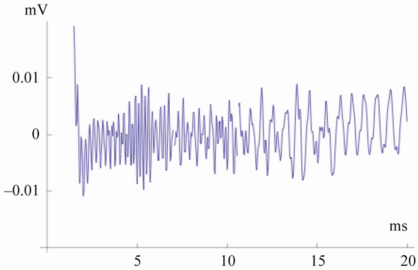
Panels (a) and (b) of Figure 2 show the output of the electronic model using 128 and 64 partitions to model the cochlea, respectively, as compared to the natural signal in panel (c). The simulated signals are obtained considering the values reported in the table of Appendix. In simulated and real signals, recording starts after 2.5 ms from the initial external excitation (t = 0), to get rid of the initial ringing. In both type of signals fast oscillations last up to 20 ms, with higher frequencies having shorter latencies, in agreement with the latency-frequency relationship typical of TEOAEs [21]. The signal simulated using 128 partitions (Panel a) is in complete agreement with that of a purely analytical model reported in [22]; the signal simulated by 64 partitions (Panel b), however, appears closer to the natural TEOAEs (Panel c). This is confirmed by a spectral analysis of the three signals carried out in five subsequent and identical time windows (not shown), indicating a much higher correlation with the natural TEOAEs of the 64 partitions output. A further decrease in the number of partitions, down to 32 or 16, introduces unbearable artifacts due to discontinuity related spurious reflections in the electronic circuits, while such artifacts are absent in the 64 partitions case.
Figure 3 shows the recurrence plots corresponding to the signals in Figure 2 (in the same order). RPs were calculated as follows: time course of the original signal described by 442 points on both axes (512 - 70, to get rid of the initial ringing); delay in the embedding procedure (lag) = 1; embedding dimension = 10; cut-off distance (radius) = 15. The radius is defined as the superior threshold for a between epochs (rows of the embedding matrix) distance to be considered as recurrent. It may be noticed that even at a first sight the shape of the 64 parti-
 (a)
(a) 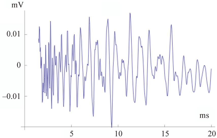 (b)
(b)  (c)
(c)
(a), (b) and (c) panels show simulations by 128 and 64 cochlear partitions, and the natural signal respectively. Both in simulated and real signals, recording starts after 2.5 ms from the initial external excitation (t = 0), to get rid of the initial ringing. Fast oscillations last up to 20 ms, with higher frequencies having shorter latencies, in agreement with the latency-frequency relationship typical of TEOAEs [24].
Figure 2. Simulated and natural TEOAs.
tions RP is closer to that of the natural signal.
Figure 4 (left) reports the points in the PC1/PC2 plane corresponding to the signals simulated changing the parameters of the middle ear according to the table of Appendix in the 64 partitions model. The position of a given point in the PC1/PC2 plane changes when the value of a parameter of the middle ear is changed, but it still remains well inside the NA circle. In terms of biological
 (a)
(a)  (b)
(b) 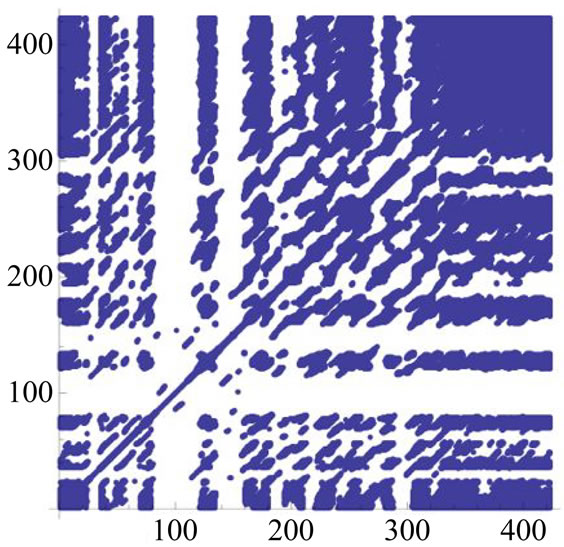 (c)
(c)
The three panels show the RPs corresponding to the signals in Figure 2, in the same order.
Figure 3. Recurrence Plots of simulated and natural signals
relevance, such indication goes beyond the simple reproduction of a “typical” signal, which actually does not exist but as an abstraction. Avan and coworkers [23] explicitly comment on this by noting the marked variability of TEOAEs. Using the 128 partitions model (Figure 4, right), still many simulated signals are inside the “physiological circle”, but their distribution is quite different and strongly biased toward the extreme left of the circle, pointing to a less natural variability distribution. Notice that the two couples of points marked by white symbols, corresponding to the rows marked by asterisks in the
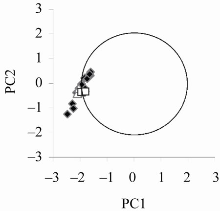
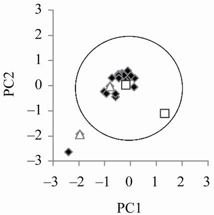
The left and right panels refer to simulations performed with the 64 and 128 partition model, respectively, and the set of parameters for the middle ear listed in the Appendix. The simulated signals have been analyzed by RQA and the resulting parameters submitted to PCA. The two couples of white symbols (triangles and squares) correspond to identical set of parameters in the two panels, marked by asterisks in the Appendix.
Figure 4. Simulated individual variability of TEOAE.
table of Appendix are more distant between each other in the left than in the right panel. This is an indication of the higher resolution power of the 64 partition model, that adds to the more natural shape of between signals variability.
4. Discussion and Conclusions
In this paper the ear model developed by Giguere and Woodland [7,8] was solved using the PSpice simulator. This model is inspired to the so called travelling wave mechanism, that is by no means the only accepted mechanism of cochlear functions. However, the point here is not to compare alternative explanations of the physical mechanism at the basis of hearing: we hope to provide a useful hypotheses-generating workbench of noticeable physical appeal, which needs confirmation in the appropriate clinical context.
Our modeling approach lies somewhere in the middle between purely phenomenological models, where the main emphasis is on fitting the shape of natural signals, and models inspired by strong hypotheses on the driving forces at the basis of the observed phenomena. The middle way approach proved powerful in many biological problems ranging from protein sequence-structure relations [24] to the rationalization of gene expression dynamics in terms of attractors [25], to the synchronization of cellular activity in the form of spiral waves causing heart contraction [26].
The success of such models stems from their peculiar interest in reproducing the biological variability (in our case the differences among natural TEOAEs) more than the ideal functioning of the system at hand. In fact, in a set of biological elements (being protein sequences, physiological signals or gene expression profiles) the differences between elements constitute more stable and relevant observations than difficult to identify “ideal cases”. Purely phenomenological approaches appear well suited for the analysis of biological variability, thanks to their main data fitting nature. However, they are of little or no use for deriving useful hypotheses on the actual system functioning and they can only be used for empirical comparisons, e.g. the receptor binding efficiency of a drug [27]. The middle layer strategy, on the other hand, allows for an analogy between single elements of the model and the corresponding elements of the real system. In our case we demonstrated that model variations due to changes in the middle ear provoked a realistic variability of the corresponding simulated signals, thus indicating the middle ear as an anatomical structure responsible for TEOAEs variations.
Both phenomenological and physically intensive models are expected to have a monotonically increasing relation between accuracy and model complication simply due to statistical considerations. More degrees of freedom allow for a greater flexibility and consequent adaptation power in the case of phenomenological approaches, and for a higher level of detail in the case of mechanistically intensive (realistic) models. In both cases, however, the risk is that the accuracy increase will be eventually paid for in terms of over-fitting and consequent degradation of the models when applied to different data sets. After a certain accuracy, in fact, phenomenological models start to model “noise”, while mechanistically intensive approaches assume not sufficiently known (and thus unjustified) details. The situation is different for “middle layer” approaches where the optimal accuracy is usually reached at a specific detail scale. This was particularly evident in the case of heart cells synchronization where the two dimensional spiral wave model gave much more reliable results than the three dimensional scroll wave analogue [26], even if the heart is a three-dimensional object. In our case the clear superiority of 64 partitions model with respect to the 128 one indicates that the identification of the over 3000 functional modules present in the Organ of Corti with the partitions of the model does not hold, and that the realism (in terms of reproduction of natural variability) of the model emerges from a reduction of the active degrees of freedom of the system, possibly due to the high level of coupling of its elements. As a matter of fact, our results confirm the spectral coding of sounds in the cochlea by way of less than 40 independent filters [28].
We believe that reproducing the physiological variability instead of often unrealistic ideal cases is a desirable goal in modeling biological phenomena. In such a context, considering the non obvious correlation between model complication and heuristic power can greatly enhance the relevance of physical models.
5. Acknowledgements
We thank Dr. C. Parlapiano of the Palermo University (Audiology Department) for having made available the TEOAEs signals
REFERENCES
- D. T. Kemp, “Stimulated Acoustic Emissions from within the Human Auditory System,” Journal of the Acoustical Society of America, Vol. 64, No. 5, 1978, pp. 1386-1391. doi:10.1121/1.382104
- G. Zimatore, A. Giuliani, C. Parlapiano, G. Grisanti and A. Colosimo, “Revealing Deterministic Structures in Click-Evoked Otoacoustic Emissions,” Journal of Applied Physiology, Vol. 88, No. 4, 2000, pp. 1431-1437.
- G. Zimatore, S. Hatzopoulos, A. Giuliani, A. Martini and A. Colosimo, “Comparison of Transient Otoacoustic Emission Responses from Neonatal and Adult Ears,” Journal of Applied Physiology, Vol. 92, No. 6, 2002, pp. 2521-2528.
- L. Robles and M. Ruggero, “Mechanics of the Mammalian Cochlea,” Physiological Reviews, Vol. 81, No. 3, 2001, pp. 1305-1352.
- H. Wit, P. van Dijk and P. Avan, “Wavelet Analysis of Real Ear and Synthesized Click-Evoked Otoacoustic Emissions,” Hearing Research, Vol. 73, No. 2, 1994, pp. 141-147. doi:10.1016/0378-5955(94)90228-3
- R. Lyon and C. Mead, “An Analog Electronic Cochlea,” IEEE Transactions on Acoustic Speech, Signal Processing, Vol. 36, No. 7, 1988, pp. 1119-1134.
- C. Giguere and P. Woodland, “A Computational Model of the Auditory Periphery for Speech and Hearing Research. i) Ascending Path,” Journal of the Acoustical Society of America, Vol. 95, No. 1, 1994, pp. 331-342. doi:10.1121/1.408367
- C. Giguere and P. Woodland, “A Computational Model of the Auditory Periphery for Speech and Hearing Research. ii) Descending Path,” Journal of the Acoustical Society of America, Vol. 95, No. 1, 1994, pp. 343-349. doi:10.1121/1.408367
- J. Merhaud, “Theory of Electroacoustics,” McGraw-Hill, New York, 1981.
- C. Shera, Tubis and C. Talmadge, “Do forwardand Backward-Traveling Waves Occur within the Cochlea? Countering the Critique of Nobili et al.,” JARO—Journal of the Association for Research in Otolaryngology, Vol. 5, No. 4, 2004, pp. 349-359. doi:10.1007/s10162-004-4038-1
- M. Gardner and M. Hawley, “Network Representations of the External Ear,” Journal of the Acoustical Society of America, Vol. 52, No. 6B, 1972, pp. 1620-1628. doi:10.1121/1.1913295
- M. Lutman and A. Martin, “Development of an Electroacoustic Analogue Model of the Middle Ear and Acoustic Reflex,” Journal of Sound and Vibration, Vol. 64, No. 1, 1979, pp. 133-157. doi:10.1016/0022-460X(79)90578-9
- M. Suesserman and F. Spelman, “Lumped-Parameter Model for in Vivo Cochlear Stimulation,” IEEE Transactions on Biomedical Engineering, Vol. 40, No. 3, 1993, pp. 237-245. doi:10.1109/10.216407
- J. Eckmann, S. Kamphorst and D. Ruelle, “Recurrence Plots of Dynamical Systems,” Europhysics Letters, Vol. 4, No. 9, 1987, pp. 973-977. doi:10.1209/0295-5075/4/9/004
- C. Webber and J. Zbilut, “Dynamical Assessment of Physiological Systems and States using Recurrence Plot Strategy,” Journal of Applied Physiology, Vol. 76, No. 2, 1994, pp. 965-973.
- A. Giuliani, G. P. V. Marigliano and A. Colosimo, “A Non-Linear Explanation of Aging-Induced Changes in Heartbeat Dynamics,” American Journal of Physiology, Vol. 275, 1998, pp. H1455-H1461.
- A. Giuliani and C. Webber, “Recurrence Quantification Analysis and Principal Components in Detection of Short Complex Signals,” Physical Letters A, Vol. 237, No. 3, 1998, pp. 131-135. doi:10.1016/S0375-9601(97)00843-8
- A. Giuliani, R. Benigni, J. Zbilut, P. Sirabella and A. Colosimo, “Nonlinear Methods in the Analysis of Protein Sequences: A Case Study in Rubredoxins,” Biophysical Journal, Vol. 78, No. 1, 2000, pp. 136-149. doi:10.1016/S0006-3495(00)76580-5
- N. Marwan, M. Romano, M. Thiel and J. Kurths, “Recurrence Plots for the Analysis of Complex Systems,” Physics Reports, Vol. 438, No. 5-6, 2007, pp. 237-329. doi:10.1016/j.physrep.2006.11.001
- G. Zimatore, S. Hatzopoulos, A. Giuliani, A. Martini and A. Colosimo, “Otoacoustic Emissions at Different Click Intensities: Invariant and Subject Dependent Features,” Journal of Applied Physiology, Vol. 95, 2003, pp. 2299- 2305.
- G. von Bekesy, “Experiment in Hearing,” McGraw-Hill Inc., New York, 1960.
- L. Zheng, Y. Zhang, F. Yang and D. Ye, “Synthesis and Decomposistion of Transient-Evoked Otoacoustic Emissions based on an Active Auditory Model,” IEEE Transactions on Biomedical Engineering, Vol. 46, No. 9, 1999, pp. 1098-1105. doi:10.1109/10.784141
- P. Avan, B. Buki, B. Maat, M. Dordain and H. P. Wit, “Middle Ear Influence on Otoacoustic Emissions,” Hearing Research, Vol. 140, No. 1-2, 2000, pp. 189-201. doi:10.1016/S0378-5955(99)00201-4
- A. Giuliani, R. Benigni, J. Zbilut, C. Webber, P. Sirabella and A. Colosimo, “Nonlinear Signal Analysis Methods in the Elucidation of Protein Sequence/Structure Relationships,” Chemical Reviews, Vol. 102, No. 5, 2002, pp. 1471-1491. doi:10.1021/cr0101499
- S. Huang, “Reprogramming Cell Fates: Reconciling Rarity with Robustness,” BioEssays, Vol. 31, No. 5, 2009, pp. 546-560. doi:10.1002/bies.200800189
- A. Winfree, “The Geometry of Biological Time,” Springer, Berlin, Heidelberg, 2000.
- P. Munson and D. Rodbard, “LIGAND: A Versatile Computerized Approach for Characterization of Ligand-binding Systems,” Analytical Biochemistry, Vol. 107, No. 1, 1980, pp. 220-239. doi:10.1016/0003-2697(80)90515-1
- B. Moore, “Coding of Sounds in the Auditory System and Its Relevance to Signal Processing and Coding in Cochlear Implants,” Otology and Neurotology, Vol. 24, No. 2, 2003, pp. 243-254. doi:10.1097/00129492-200303000-00019
Appendix
1. Principal Component Analysis
Principal Component Analysis (PCA), is a quite common statistical technique able to project a multivariate data set into a space of orthogonal axes, called principal components (PCs) and correspondent to the eigenvectors of the covariance (or correlation) matrix between the original variables. PCs are selected, one after the other (PC1, PC2, etc.), on the basis of the maximal variance explained in the space of the original variables. The presence of nonnull correlations allows to reduce the data set dimension in the new space without noticeable loss of information.
Because PCs are, by construction, orthogonal to each other, a separation of the different and independent features characterizing the data set is possible.
2. Table: Middle Ear Parameters for Simulated TEOAEs
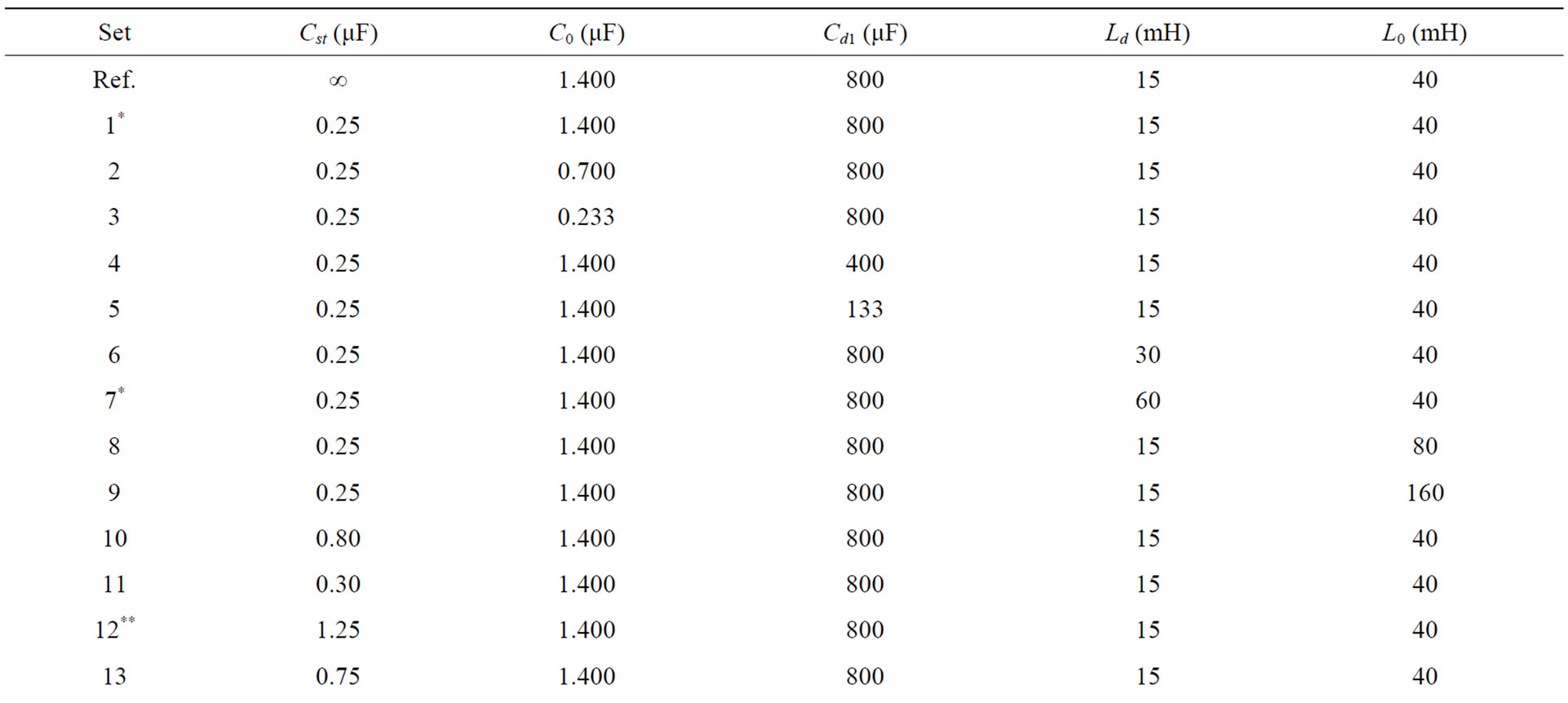
TEOAEs signals were simulated by the electric model in Figure 1. For the meaning of the symbols see the text and Figure 1. The reference values (Ref) are from [7]. Rows 1*, 7* and rows 12**, 16** refer to the maximal excursion of  and
and , respectively (see Figure 4 Left, Right).

NOTES
*Corresponding author.