Journal of Power and Energy Engineering
Vol.2 No.5(2014), Article ID:46169,12 pages DOI:10.4236/jpee.2014.25002
A Stable Energy Saving Adaptive Control Scheme for Building Heating and Cooling Systems
Sumera I. Chaudhry, Manohar Das
Department of Electrical and Computer Engineering, Oakland University, Rochester, USA
Email: sichaudh@oakland.edu, das@oakland.edu
Copyright © 2014 by authors and Scientific Research Publishing Inc.
This work is licensed under the Creative Commons Attribution International License (CC BY).
http://creativecommons.org/licenses/by/4.0/


Received 5 March 2014; revised 5 April 2014; accepted 12 April 2014
ABSTRACT
This paper presents a stable, nonlinear, adaptive control scheme for building heating and cooling systems. The proposed controller utilizes the principle of adaptive one step ahead control and aims at reducing the energy consumed for heating or cooling a building. The design steps are discussed in details and a proof of global stability is also provided. Also, the performance of the proposed controller is demonstrated on a simulated building thermal model.
Keywords:Building HVAC Control, Adaptive Control, Energy Saving Control

1. Introduction
According to EPA estimates, the cost of heating, ventilation and cooling (HVAC) of residential and commercial buildings constitute about 50% of the total electrical energy consumed in USA. Thus, minimization of this HVAC energy consumption can be very beneficial not only because of the resulting cost savings but also because of the reduction of carbon footprints of buildings. In recent years, the installation of smart meters in buildings and advent of smart grid technology have provided an impetus to development of advanced control schemes for reducing the energy consumption and maintaining the thermal comfort inside a building. A variety of such advanced control schemes have appeared in the literature [1] -[7] . Some of these claim to be adaptive, efficient, and helpful in reducing the energy consumption while maintaining the occupants’ comfort level. Examples include classical PID controller and PID plus fuzzy logic controller [1] [2] , optimal, adaptive and intelligent controllers [2] , adaptive neuro-fuzzy inference system (ANFIS) and artificial neural network (ANN) based controllers, and fuzzy logic (FL) controllers [3] . Also, other approaches include model predictive control (MPC) [4] [5] , and predicted mean vote (PMV) based adaptive or PID controller [6] -[8] . Till this date, however, very little efforts have been made in employing truly adaptive techniques that learn the nonlinear thermal characteristics of a building and its environment, and presenting a nonlinear adaptive controller backed up by a proof of globally stability. This paper is aimed at addressing these concerns.
Notice that adaptive controllers are ideally suited for controlling the heating/cooling system of a building, because such controllers can estimate the building’s physical parameters and occupancy levels online and adjust the control signals accordingly. The main difficulty in designing such controllers stems from the fact that a building thermal system is usually characterized by a bilinear model. In view of this, we investigate the application of adaptive one step ahead (OSA) and weighted one step ahead (WOSA) control schemes [9] here, because such controllers are easy to design and capable of controlling both linear and bilinear systems quite well. The contributions of this paper are threefold. First we investigate in details the application of adaptive one step a head (OSA) and weighted one step ahead (WOSA) control schemes for controlling the thermal system of a building. Then we investigate the criteria for global stability of the closed loop system, and present a detailed proof of the same. Finally, we present results of a simulation study that compares the performance of the adaptive OSA and WOSA controllers with that of a simple fuzzy control scheme, and show that OSA and WOSA controllers are capable of reducing the heating/cooling energy consumption in a building.
The organization of this paper is as follows. Section 2 presents a brief overview of the objectives and methodology. A dynamical model of a building’s thermal system is described briefly in Section 3. A description of OSA and WOSA controllers and a discussion of parameter estimation issues are presented in Section 4. A detailed proof of global stability of the closed loop system is presented in Section 5. Then Section 6 presents results of some simulation studies, and finally, some concluding remarks are given in Section 7.
2. An Overview of Objectives and Methodology
The aim of this paper is to present a scheme for controlling the indoor temperature of a building in a desired way using a globally stable control scheme that also exhibits good tracking. Such a controller is based on a simple nonlinear dynamical model of the thermal system of a building. The parameters can be different for different buildings and can be time varying, and in most cases we have no knowledge of the parameter values. Therefore, due to the nonlinear nature of the dynamical model and the unknown parameters, an adaptive control approach is used to fulfill the objective.
The goal of a smart building temperature control system is to maintain the indoor temperature of a building by achieving an optimum tradeoff between heating/cooling energy consumption and occupants’ comfort. The overall heating/cooling energy consumed in a building can be divided into two parts: 1) energy consumed to maintain the current conditions, and 2) energy consumed to raise (or lower) temperature to a different level. The latter becomes an important part of the overall energy saving strategy because during favorable outdoor conditions, periods of low occupancy levels and at nights, the target temperature can be lowered (during winter season) or raised (during summer season) to save energy, and subsequently brought back to the desired level whenever desired. However, in doing so, the reference temperature profile needs to be chosen carefully by avoiding steep gradients (to reduce energy consumption) and at the same time maintaining a desired comfort level. The proposed adaptive control scheme involves measurement of inputs and outputs of the system, estimation of unknown system parameters using a recursive least squares (RLS) parameter estimation algorithm, and computation of a control signal based on the estimated parameter values. The design of both OSA and WOSA controllers is discussed and their performance is studied.
3. Dynamical Model of a Building’s Thermal System
At the outset, it should be noted that since the heating and cooling dynamics are very similar, we discuss only the heating dynamics here for the sake of brevity. Following the footsteps of Calvino et al. [7] and IBPT toolbox [10] , a simplified dynamical model of a building’s thermal system during a heating season can be described by the following equation:
 (1)
(1)
where  denotes the indoor air temperature at time t,
  is the outdoor air temperature at time t,
  denotes the total heat capacity of the indoor air mass and other objects inside the building,
 ![]() is the specific heat of the warming carrier,
is the specific heat of the warming carrier,  denotes the temperature difference between the inlet and outlet ends of the heat exchanger, and
  denotes the difference between the average temperature of the heating medium and the indoor air temperature. Also, HT denotes the global heat transfer coefficient of the building envelope and
  denotes the heat gains from various internal and external sources. A more detailed description of the above terms can be found in references [7] and [10] .
Before presenting our control strategies, it would be convenient to make the following changes of variables for the sake of notational simplicity:

Thus, Equation (1), which represents a simplified dynamical model of the building, now takes the following form:
 (2)
(2)
where y(t) denotes the indoor temperature, u(t) is the flow rate of the warming carrier and A, B and C denote the model parameters that are given by:
 (3a)
(3a)
 (3b)
(3b)
 (3c)
(3c)
As considered in [1] , we assume that the thermal losses due to ventilation are insignificant, but the convective part of all heat sources, such as the solar heat gains and the heat gains from the heating system or casual gains, are considered to be parts of the model equation. The following discrete time equation is derived from the system Equation (1) using a first order Euler approximation for  with a sampling period Ts.
 (4)
(4)
where k denotes the discrete time index (i.e., ) and the time instance,
  , is simply denoted by k. The above thermal model is characterized by three unknown parameters, namely, A, B and C.
4. Control of Indoor Temperature of a Building
To develop a control scheme for controlling the indoor temperature of a building governed by Equation (4), first thing to notice is that it represents a nonlinear system characterized by some unknown parameters. These parameters can vary from building to building, and in most cases we have no prior knowledge of the parameter values. In view of this, we propose to use a nonlinear, adaptive OSA and WOSA controllers [9] . Furthermore, it is important to establish that the resulting closed loop system is stable and exhibits good tracking behavior.
The proposed adaptive control scheme involves measurement of inputs and outputs of the system, estimation of unknown system parameters using a recursive least squares (RLS) parameter estimation algorithm, and computation of a control signal based on the estimated parameter values. First the design of fixed OSA and WOSA controllers is discussed and their performance is studied.
4.1. Fixed One Step Ahead Control Algorithm
The goal of a fixed OSA controller is to track a desired reference temperature profile, . Such a tracking is achieved by bringing the predicted output at time k + 1, i.e.,
  , to the desired value,
  in one step. The feedback control law that achieves this goal is found by minimizing the following cost function based on a squared prediction error:
 (5)
(5)
The discrete time control law, obtained by differentiating  with respect to u(k) and setting it to zero, is given by [9] :
 (6)
(6)
However, in view of the fact that any furnace is limited by its maximum heat delivery capacity, it is necessary to constrain the above control signal,  , and generate a constrained control signal, u(k), as follows:
 if
if  (7a)
(7a)
else  if
if  (7b)
(7b)
else  if
if  (7c)
(7c)
where  denotes the maximum low rate of the warming carrier.
4.2. Fixed Weighted One Step Ahead Control Algorithm
Since OSA controllers attempt to achieve zero tracking error in one step, they often require large control efforts, u(k), which usually increases the overall energy consumption. To alleviate this drawback, a weighted OSA (WOSA) controller [9] is often found to be a good alternative. A WOSA controller attempts to achieve a tradeoff between tracking error and control efforts. It minimizes the following cost function:
 (8)
(8)
where the parameter, ![]() , controls the trade-off between tracking error and control efforts. A larger
, controls the trade-off between tracking error and control efforts. A larger ![]() reduces control efforts at the cost of higher tracking error and vice versa.
reduces control efforts at the cost of higher tracking error and vice versa.
The control law that minimizes  is given by [9] :
 (9)
(9)
which is once again constrained by  to generate a constrained control signal, u(k), defined by Equations (7a)-(7c).
4.3. Adaptive OSA and WOSA Controllers
In an adaptive controller, the sampled measurements, u(k) and y(k), are used to estimate the model parameters, A, B and C in Equation (2), using a recursive parameter estimation method, such as recursive least squares (RLS). The estimated values of theses parameters are then used to compute the OSA/WOSA control signals.
4.3.1. Parameter Estimation
First we write model Equation (2) in the following form:
 (10)
(10)
where
 (11a)
(11a)
 (11b)
(11b)
Next, the estimated value of ![]() is computed recursively using the following RLS algorithm:
is computed recursively using the following RLS algorithm:
 (12a)
(12a)
 (12b)
(12b)
 (12c)
(12c)
 (12d)
(12d)
where γ > 0 is a small number and σ > 0 is chosen to be large. Also,  is always constrained to be nonnegative by using a projection algorithm [9] , i.e.,
 (12e)
(12e)
Given an estimate  of
of![]() , we define the predicted output at time k + 1 as:
, we define the predicted output at time k + 1 as:
 (13)
(13)
4.3.2. Adaptive Control Algorithms
The adaptive OSA and WOSA controllers use the above estimate,  , to compute the control signal, u(k), from the following adaptive versions of Equations (6) and (9):
For OSA:
 (14)
(14)
For WOSA:
 (15)
(15)
where ,
,  and
and  denote the estimated values of A, B and C, respectively, at time k.
5. Global Stability of the Closed Loop Adaptive Control System
A proof of global stability of the closed loop system governed by adaptive OSA controller is provided in this section under the following mild assumptions:
Assumption 1 The building thermal parameters, A, B and C have finite, positive values, i.e.,


Assumption 2 The room temperature, y(k), is always less than the average temperature, yfav, of the heat exchanger, i.e., for all k.
The global stability of the closed loop system can now be established by first proving three Lemmas and finally proving Theorem 1 below.
Lemma 1 For the least squares algorithm describes by Equations (12a)-(12d), we have
 (16a)
(16a)
 (16b)
(16b)
where a1 is some constant and prediction error, e(k), is given by
 (16c)
(16c)
Proof The proof of Lemma 1 can be found in Goodwin and Sin [9] .
Next the boundedness of y(k) is proved in Lemma 2 below.
Lemma 2 Consider the closed loop adaptive OSA control system governed by Equations (2), (14) and (7a)-(7c). This system is BIBO stable and therefore, y(t) is bounded for all t.
Proof Notice that at any , the closed loop system governed by Equation (2) can be rewritten as:
 (17)
(17)
where , which is given by Equations (14) and (7a)-(7c), and α(t) is defined as
 (18)
(18)
In view of (7a)-(7c) and assumptions 1 and 2, we get
 (19a)
(19a)
 (19b)
(19b)
First consider the homogeneous system associated with Equation (17), i.e.,
 (20)
(20)
The state transition matrix [11] of this homogeneous system is given by
 (21)
(21)
In view of (19b), we have
 (22)
(22)
In view of (22), the homogeneous system given by Equation (20) is uniformly asymptotically stable [11] .
Next, consider the closed loop system given by Equation (17). Since its homogeneous system described by (20) is uniformly asymptotically stable and the excitation given by the right hand side of Equation (17) is bounded for all times (in view of Assumption 1 and Equation (19a)), the system governed by (17) is BIBO stable [14] . This implies y(t) is bounded for all t. Next, the following Lemma establishes the boundedness of the prediction error, e(k), defined by Equation (16c).
Lemma 3
 (23)
(23)
Proof In view of Equation (19a) and Lemma (2), the regression vector,  defined by Equation (11a) is bounded, i.e.,
 (24)
(24)
where M1 is some constant. In view of Equation (16b) of Lemma 1 and (24), we get (23). Finally, a tracking result is provided in Theorem 1 below.
Tracking In order to prove tracking properties of the adaptive OSA controller, we are going to assume (for the sake of simplicity) that  is a constant,
![]() . Notice that this is a reasonable assumption because
. Notice that this is a reasonable assumption because  is actually piecewise constant for all t.
Theorem 1 Subject to the assumptions 1 and 2, the proposed adaptive OSA scheme assures that
 (25)
(25)
Proof We present an outline of the proof here, because it is very similar to the results presented in [12] [13] and details can be found there. First of all, notice that from Lemma 1, we get
 (26)
(26)
Thus, for a given η, there exists a ![]() such that for
such that for ,
,
 (27)
(27)
Define an interval,
 (28)
(28)
From here on we assume  and proceed to consider the following three possible cases for u(k) given by (28) and (7a)-(7c):
(i)  for
for ,
, 
(ii)  for
for ,
, 
(iii)  for
for ,
, 
First we show that there exists a  such that
 (29)
(29)
Case (i) If (i) holds, then  and clearly
 . Similarly,
  ,
, 
Case (ii). If (ii) holds, then Equation (7c) implies . This, in view of (14), yields
 ,
, . Thus, Equation (27) yields
 . But u(k) = 0 means furnace is off, which implies
  decreases asymptotically to a steady state value determined by the outdoor temperature,
 . Thus, there exists a
  such that
  Thus,
Thus, . However, if the above sequence,
  terminates at time
  before
 , then furnace turns on, which returns us to case (i) and therefore,
 .
.
Case (iii). If (iii) holds, then y(k) increases due to heat output from the furnace. But  implies (from (7b))
 . This, in view of (14), yields
 ,
, . Thus, Equation (27) yields
 ,
, . In a similar fashion like in case (ii), we can once again prove that there exists a
  such that
  for
for .
.
From here on, by induction on (29), it follows that  for some
 . Finally, since
 ![]() can be chosen arbitrarily, the above result also establishes (25).
can be chosen arbitrarily, the above result also establishes (25).
Remarks 1) In the above analysis, noise is assumed to be absent. In presence of bounded noise, the analysis can be modified slightly and following arguments similar to [12] [13] , it can be shown that there exists a  such that for
 (30)
(30)
where  for all times.
2) For the adaptive OSA, the tracking error is zero, whereas for the adaptive WOSA, the tracking error is proportional to the weight, λ, and inversely proportional to the square of the sampling time , which can be shown easily by substituting control u(k) in the equation for y(k).
6. Simulation Results and Discussion
In this section, we present results of a simulation study to show the performance of OSA and WOSA controllers and also compare them with a simple fuzzy logic controller. These simulations are conducted on a simplified thermal dynamical model of a small family home that was studied by Calvino et al. [7] . However, in our case, this home is assumed to be located in Michigan, USA. The physical parameters of this home are assumed to be Table 1.
The simulations are carried out over a period of 24 hours, or equivalently 86,400 seconds. The outdoor temperature during this period is assumed to vary slowly in a sinusoidal fashion as follows:
 (31)
(31)
which represents the outdoor temperature variation on a typical winter day in Michigan, USA. However, the desired indoor temperature profile, y*(t), is assumed to be just a two-level signal consisting of a low level and a high level. It is set to be at the high level during early morning and evening hours, whereas it is lowered to the low-level setting during night time as well as office hours when the place is devoid of occupants.
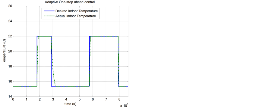
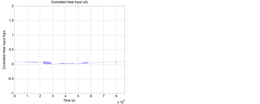
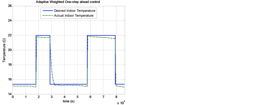
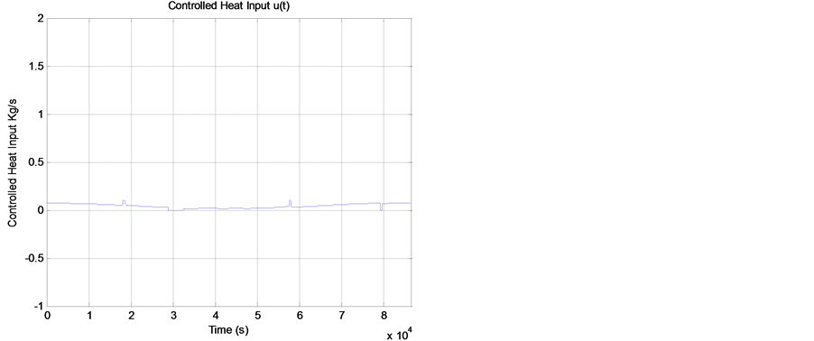
The performance of an adaptive OSA controller is depicted in Figure 1 and Figure 2. These simulations were carried out using two different values of maximum blower speed (umax) of the furnace, 0.1 Kg/sec and 0.5 Kg/sec. Figure 1(a) and Figure 1(b) compare the actual indoor temperature with the desired one for the above settings of umax. Although both show good tracking between the actual temperature and the desired one, we notice that the furnace with a higher umax results in a faster rise of the actual temperature. Figure 2(a) and Figure 2(b) depict the behavior of the control signal, u(t), in these two cases. As can be seen from these figures, the furnace with a higher umax results in a smoother control signal. However, this improvement in performance has to be traded off against a higher capital cost for the high-capacity furnace.
The performance of an adaptive WOSA controller is depicted in Figure 3 and Figure 4. Since we wish to show the effect of variation of the controller trade-off parameter, ![]() , we just use a lower capacity furnace with umax = 0.1 Kg/s for this part of the study. However, the value of
, we just use a lower capacity furnace with umax = 0.1 Kg/s for this part of the study. However, the value of ![]() is chosen to be 0.1 and 0.05, respectively, for these two case. Figure 3(a) and Figure 3(b) compare the tracking errors for the above two cases. As can be seen from these figures, a smaller value of
is chosen to be 0.1 and 0.05, respectively, for these two case. Figure 3(a) and Figure 3(b) compare the tracking errors for the above two cases. As can be seen from these figures, a smaller value of ![]() improves the tracking between the actual temperature and the desired one. Figure 4(a) and Figure 4(b) show the corresponding control signals. A comparison of these figures with Figure 4(a) and Figure 4(b) clearly shows that a WOSA controller substantially reduces the control efforts.
improves the tracking between the actual temperature and the desired one. Figure 4(a) and Figure 4(b) show the corresponding control signals. A comparison of these figures with Figure 4(a) and Figure 4(b) clearly shows that a WOSA controller substantially reduces the control efforts.
The performance of the above OSA and WOSA controllers is next compared with that of a simple fuzzy controller, described by the following equations:
 (32)
(32)
where the variables e (absolute error) and ∆e (time variation of the error) is defined as
 (33)
(33)
 (34)
(34)

Table 1 . Physical parameters of the simulated building.
 (a)
(a)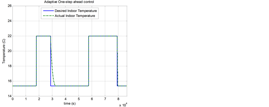 (b)
(b)
Figure 1. Comparison of actual and desired temperatures using adaptive OSA controller for (a) umax = 0.1 Kg/s and (b) umax = 0.5 Kg/s.
 (a)
(a)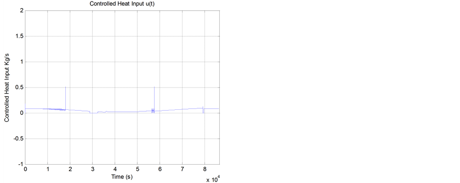 (b)
(b)
Figure 2. Behavior of adaptive OSA control signals for (a) umax = 0.1 Kg/s and (b) umax = 0.5 Kg/s.
 (a)
(a)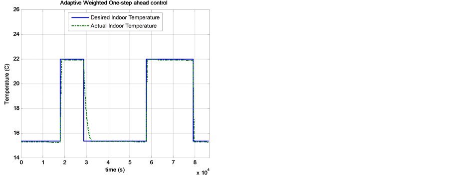 (b)
(b)
Figure 3. Comparison of actual and desired temperatures using adaptive WOSA controller for (a) λ = 0.05 and (b) λ = 0.01.
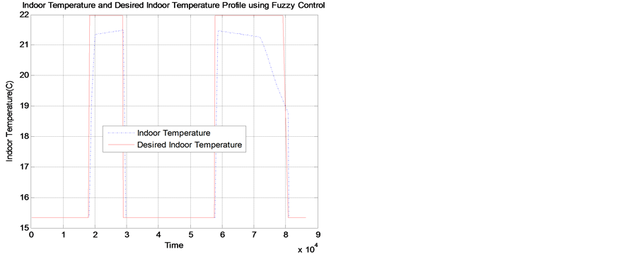
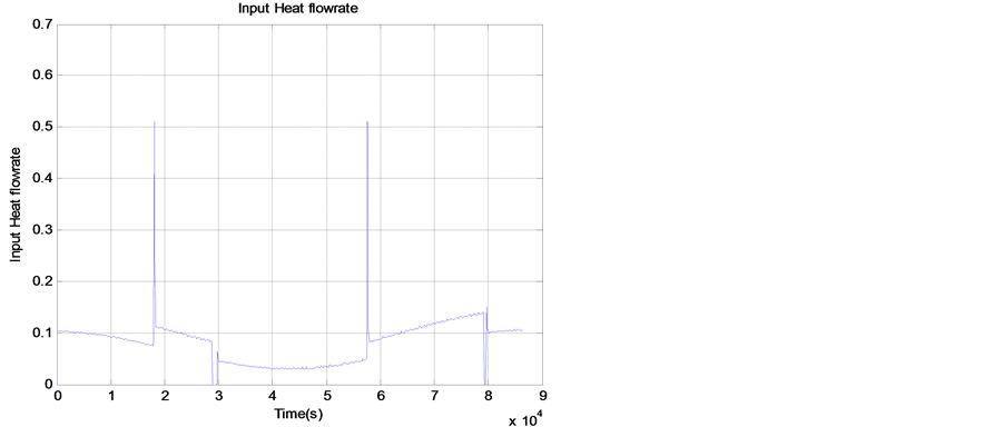
A fuzzy controller, consisting of 25 Sugeno-style decision rules, was designed using Matlab fuzzy logic toolbox and used in this part of our study. The performance of the above controller is depicted in Figure 5 and Figure 6. Figure 5(a) shows the tracking performance for umax = 0.1 Kg/seccc, which seems to be rather poor. The controller is unable to track the desired temperature profile because of the lower heat delivery capacity of the furnace. In view of this, umax was increased to 0.5 Kg/sec to see if it would improve the tracking performance. As shown in Figure 5(b), this indeed is the case, but the overall tracking performance is not as good as adaptive OSA and WOSA controllers. Figure 6(a) and Figure 6(b) depict the behavior of the control signals for the above two cases.
Finally, the energy consumptions of OSA, WOSA and fuzzy controllers using same reference temperature profile are compared in Table 2. It is evident from this table that both OSA and WOSA controllers can deliver significant energy savings per day, which becomes even more significant when the total number of cold days in a winter season is taken into consideration.
7. Conclusion
An adaptive one-step ahead control scheme and a weighted one-step ahead control scheme for a building’s
 (a)
(a) (b)
(b)
Figure 4. Behavior of adaptive WOSA control signals for (a) λ = 0.05 and (b) λ = 0.01.
 (a)
(a)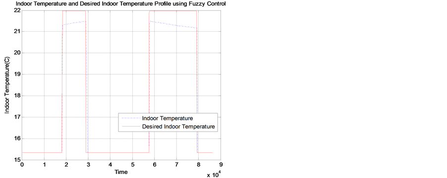 (b)
(b)
Figure 5. Comparison of actual and desired temperatures using a simple fuzzy controller for (a) umax= 0.1 Kg/s and (b) umax = 0.5 Kg/s.
Table 2. Comparison of energy consumption/day for Fuzzy, OSA and WOSA controllers.
 (a)
(a)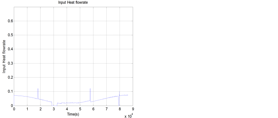 (b)
(b)
Figure 6. Behavior of fuzzy control signal for (a) umax = 0.1 Kg/s and (b) umax = 0.5 Kg/s.
HVAC systems are presented in this paper. A proof of global stability of the closed-loop system for the adaptive OSA controller is also presented. The performance of the proposed controllers is compared with that of a fuzzy-logic controller. The results of some simulation studies show that the adaptive OSA and WOSA controllers deliver better performance in terms of both tracking the desired temperature profile and reducing the overall energy consumption as compared to the Fuzzy controller. Further reduction of energy consumption by utilizing an optimized reference temperature profile is currently under investigation.
References
- Jimenez, M.J., Madsen, H. and Andersen, K.K. (2008) Identification of the Main Thermal Characteristics of Building Components Using Matlab. Building and Environment, 43, 170-180. http://dx.doi.org/10.1016/j.buildenv.2006.10.030
- Paris, B., Eynard, J., Grieu, S., Talbert, T. and Polit, M. (2010) Heating Control Schemes for Energy Management in Buildings. Energy and Buildings, 42, 1908-1917. http://dx.doi.org/10.1016/j.enbuild.2010.05.027
- Dounis, A.I. and Caraiscos, C. (2009) Advanced Control Systems Engineering for Energy and Comfort Management in a Building Environment—A Review. Renewable and Sustainable Energy Reviews, 13, 1246-1261. http://dx.doi.org/10.1016/j.rser.2008.09.015
- Moon, J.W., Jung, S.K., Kim, Y. and Han, S.H. (2011) Comparative Study of Artificial Intelligence Based Building Thermal Control Methods—Application of Fuzzy, Adaptive Neuro-Fuzzy Inference System, and Artificial Neural Network. Applied Thermal Engineering, 31, 2422-2429. http://dx.doi.org/10.1016/j.applthermaleng.2011.04.006
- Balan, R., Cooper, J., Chao, K.M., Stan, S. and Donca, R. (2011) Parameter Identification and Model Based Predictive Control of Temperature inside a House. Energy and Building, 43, 748-758. http://dx.doi.org/10.1016/j.enbuild.2010.10.023
- Ma, Y., Borrelli, F., Hencey, B., Coffey, B., Bengea, S. and Haves, P. (2010) Model Predictive Control for the Operation of Building Cooling Systems. IEEE Transactions on Control Systems Technology, 20, 796-803.
- Calvino, F., Gennusa, M.L., Morale, M., Rizzo, G. and Scaccianoce, G. (2010) Comparing Different Control Strategies for Indoor Thermal Comfort Aimed at the Evaluation of the Energy Cost of Quality of Building. Applied Thermal Engineering, 30, 2386-2395. http://dx.doi.org/10.1016/j.applthermaleng.2010.06.008
- Orosa, J.A. (2011) A New Modeling Methodology to Control HVAC Systems. Expert Systems with Applications, 38, 4505-4513. http://dx.doi.org/10.1016/j.eswa.2010.09.124
- Goodwin, G.C. and Sin, K.S. (1984) Adaptive Filtering Prediction and Control. Prentice-Hall, Englewood Cliffs.
- IBPT (2012) International Building Physics Toolbox in Simulink. http://www.ibpt.org/
- Antsaklis, P.J. and Michel, N.A. (2007) A Linear Systems Primer. Birkhauser (Springer), New York.
- Dochain, D. and Bastin, G. (1984) Adaptive Identification and Control Algorithms for Nonlinear Bacterial Growth Systems. Automatica, 20, 621-634. http://dx.doi.org/10.1016/0005-1098(84)90012-8
- Goodwin, G.C., McInnis, B. and Long, R.S. (1982) Adaptive Control Algorithms for Waste Water Treatment and pH Neutralization. Optimal control Applications and Methods, 3, 443-459.
- Fanger, P.O. (1972) Thermal Comfort: Analysis and Applications in Environmental Engineering. McGraw-Hill, New York.