Journal of Applied Mathematics and Physics
Vol.2 No.7(2014), Article ID:46803,38 pages
DOI:10.4236/jamp.2014.27056
The Mathematics of Harmony, Hilbert’s Fourth Problem and Lobachevski’s New Geometries for Physical World
Alexey Stakhov1, Samuil Aranson2
1International of the Golden Section, Academy of Trinitarism, Moscow, Russia
2Russian Academy of Natural History, Moscow, Russia
Email: goldenmuseum@rogers.com, saranson@yahoo.com
Copyright © 2014 by authors and Scientific Research Publishing Inc.
This work is licensed under the Creative Commons Attribution International License (CC BY).
http://creativecommons.org/licenses/by/4.0/


Received 26 January 2014; revised 26 February 2014; accepted 5 March 2014
ABSTRACT
We suggest an original approach to Lobachevski’s geometry and Hilbert’s Fourth Problem,
based on the use of the “mathematics of harmony” and special class of hyperbolic
functions, the so-called hyperbolic Fibonacci (-functions, which are based on the
ancient “golden proportion” and its generalization, Spinadel’s “metallic proportions.”
The uniqueness of these functions consists in the fact that they are inseparably
connected with the Fibonacci numbers and their generalization― Fibonacci (-numbers
(( > 0 is a given real number) and have recursive properties. Each of these new
classes of hyperbolic functions, the number of which is theoretically infinite,
generates Lobachevski’s new geometries, which are close to Lobachevski’s classical
geometry and have new geometric and recursive properties. The “golden” hyperbolic
geometry with the base
 (“Bodnar’s geometry) underlies the botanic phenomenon of phyllotaxis. The “silver”
hyperbolic geometry with the base
(“Bodnar’s geometry) underlies the botanic phenomenon of phyllotaxis. The “silver”
hyperbolic geometry with the base
 has the least distance to Lobachevski’s classical geometry. Lobachevski’s new geometries,
which are an original solution of Hilbert’s Fourth Problem, are new hyperbolic geometries
for physical world.
has the least distance to Lobachevski’s classical geometry. Lobachevski’s new geometries,
which are an original solution of Hilbert’s Fourth Problem, are new hyperbolic geometries
for physical world.
Keywords:Euclid’s Elements, “Golden” and “Metallic” Proportions, Mathematics of Harmony, Hyperbolic Fibonacci Functions, Lobachevski’s Geometry, Hilbert’s Fourth Problem

1. Introduction
Lobachevski’s hyperbolic geometry became the starting point of the modern stage in the development of mathematics. To stimulate the development of this mathematical discipline in the 20th century, David Hilbert paid special attention to the hyperbolic geometry in his 23 mathematical problems. He had formulated a special problem (Hilbert’s Fourth Problem) to find new hyperbolic geometries close to Euclidean geometry. Unfortunately, this important problem is still not resolved. Currently, most mathematicians are inclined to believe that Hilbert’s Fourth Problem has been formulated too vague what makes complicated its final solution. That is, the mathematicians of the 20 century laid the blame for the failure in the solution of this problem on Hilbert himself.
At the vision of Hilbert’s Fourth Problem as vague, “the game between thought and experience” (David Hilbert) means the game between the axiomatic approach and the approach on the language of strict and simple (on Hilbert’s recommendation) formulas. In this situation, this recommendation is fully consistent with the approach to Hilbert’s Fourth Problem in terms of “Mathematics of Harmony,” which has not only scientific but also great practical importance for the natural sciences.
In this article we develop an original approach to solving Hilbert’s Fourth Problem, called “the game of hyperbolic functions.” This approach has only been possible in the 21st century, when a general theory of “harmonic” hyperbolic functions, based on the ancient “golden proportion” and its generalization, the “metallic proportions,” has been developed. The uniqueness of these functions is the fact that they are inseparably connected with the Fibonacci numbers and their generalization, Fibonacci l-numbers (l > 0 is a given real number). Each of these new classes of hyperbolic functions, the number of which is theoretically infinite, generates a new hyperbolic geometry having new geometric properties, studied in the article.
A new geometric theory of phyllotaxis has been recently developed by Ukrainian architect
Oleg Bodnar. This geometry is based on the “golden” hyperbolic functions with the
base, equal to the famous “golden proportion.” To assess the proximity of new hyperbolic
geometries to Lobachevski’s classical geometry with the base e = 2.71, the important
concept of “distance” has been introduced. It is proved that the “silver” hyperbolic
function with the base
 generates new (“silver”) hyperbolic geometry, which has minimal distance to Lobachevski’s
classical geometry. This fact allows us to put forward the hypothesis that the “silver”
hyperbolic geometry may be widespread in the real physical world.
generates new (“silver”) hyperbolic geometry, which has minimal distance to Lobachevski’s
classical geometry. This fact allows us to put forward the hypothesis that the “silver”
hyperbolic geometry may be widespread in the real physical world.
Modern mathematics begins from Euclid’s Elements, which are an inexhaustible source of new mathematical ideas and directions and led to revolutionary transformations of modern science. Let us consider two of them.
Hyperbolic geometry. The following remarkable words belong to the brilliant Russian geometer Nikolay Lobachevski:
“Mathematicians paid all their attention on the Advanced Parts of Analysis, by neglecting the origins of Mathematics and not willing to dig in the field, which they already went through and had left behind.”
Unlike many mathematicians, Lobachevski did not hesitate to “dig” into some of the unsolved problems of ancient mathematics, in particular, into the problem of Euclid’s 5th postulate and this study led him to the outstanding mathematical discovery, the creation of hyperbolic geometry [1] .
Lobachevski begins his famous “Geometric study on the theory of parallel lines” with the following words:
“In geometry, I found some imperfections, which, in my opinion, are the reason why this science until now is in the state, in which it had come to us from Euclid. I attribute to these imperfections the following: the vagueness in the first definitions of geometric quantities, the methods of measurement of these quantities, and, finally, the important gap in the theory of parallel lines.”
The history of hyperbolic geometry was accompanied with many dramatic events. The first of them is a very negative reaction of the Russian academic science on the discovery of “Kazan’s rector.” Hounding began with the negative review on Lobachevski’s work, written by the famous Russian mathematician academician Ostrogradsky. Only thanks to the support of the outstanding German mathematician Gauss, the hyperbolic geometry has got the deserved recognition among 19 century’s mathematicians. Academician Kolmogorov in his excellent book [2] pointed out that “Lobachevski’s geometry was the most important discovery of the early 19th century.”
The Mathematics of Harmony. In 2009 the International Publishing House “World Scientific” has published the book: Alexey Stakhov. The Mathematics of Harmony. From Euclid to Contemporary Mathematics and Computer Science” [3] . The publication of this book is a reflection of one of the most important trends in the development of modern science. The essence of this trend is to return back to the “harmonic ideas” of Pythagoras and Plato (the “golden ratio” and Platonic solids), embodied in Euclid’s “Elements” [4] .
The newest discoveries in chemistry and crystallography: fullerenes [5] , based on the “truncated icosahedron” (Nobel Prize-1996), and quasi-crystals [6] , based on the icosahedral or pentagonal symmetry (Nobel Prize- 2011), are brilliant confirmation of this trend.
A number of such discoveries in modern science are increasing continuously. These include: “the law of structural harmony of systems” by Edward Soroko [7] , based on the generalized golden proportions, the “law of spiral biosimmetry transformation” by Oleg Bodnar [8] -[11] , based on the “golden” hyperbolic functions. It also includes an original solution of Hilbert’s Tenth Problem [12] based on the Fibonacci numbers (the author the Russian mathematician Yuri Matiyasevich) and also a new theory of the genetic code, based on the “golden genomatrices” (the author Doctor of Physical and Mathematical Sciences Sergey Petoukhov, Moscow) [13] . These examples could go on.
Thus, the modern mathematics and theoretical natural sciences begun to widely use the “harmonic ideas” by Pythagoras, Plato and Euclid. And we have every right to talk about the “revival” of ancient Greeks’ “harmonic ideas” in modern science. This fact puts forward the problem of the revival of these ancient harmonic ideas in modern mathematics. The book [3] is the answer of contemporary mathematics to this important trend.
As is showed in [4] , the mathematics of harmony goes back in its origin to Euclid’s “Elements.” This means that Euclid’s “Elements” are the source of two mathematical directions: “hyperbolic geometry,” emerged in the 19th century, and the “mathematics of harmony,” emerged in the 21st century. As is showed in [4] , there are very interesting mathematical relationships between them. They can significantly affect the future development of hyperbolic geometry. We are talking on the following scientific results, obtained in the mathematics of harmony:
1) Fibonacci hyperbolic trigonometry, based on the “golden ratio” and Fibonacci numbers [14] -[17]
2) A new geometric theory of phyllotaxis (“Bodnar’s geometry”) [8] -[11]
3) The general theory of hyperbolic functions, based on the “metallic proportions” [18] [19]
4) The original solution of Hilbert’s Fourth Problem [19] -[23]
The present article is a continuation and development of the articles [19] -[23] . The purpose of the article is to give an overview of the formation and development of the hyperbolic geometry, starting from Euclid’s Elements. The next purpose is to give an overview of the modern theory of hyperbolic Fibonacci functions, which were obtained in the framework of the mathematics of harmony [3] , a new interdisciplinary direction of modern science. The main result is to give the improved solution of Hilbert’s Fourth Problem, which has a direct relation to the hyperbolic geometry and opens new ways in the development of mathematics and all theoretical natural sciences.
2. The Golden Ratio
2.1. The Golden Ratio in Euclid’s Elements
In Euclid’s Elements we meet the task, which later had played a great role in the development of science. This task is called the “division of line segment in extreme and mean ratio.” In the Elements this task occurs in two forms. The first form is formulated in the Proposition 11 of the Book II.
Proposition II.11. Divide a given line segment AD into two unequal parts AF and FD so that the area of the square, which is built on the larger segment AF would be equal to the area of the rectangle, which is built on the segment AD and the smaller segment FD.
Let us depict this task geometrically (Figure 1).
Thus, according to Proposition II.11, the area of the square AGHF should be equal to the area of the rectangle ABCD. If we denote the length of the larger segment AF through b (it is equal to the side of the square AGHE), and the side of the smaller segment FD through a (it is equal to the vertical side of the rectangle ABCD), then the condition for Proposition II.11 can be written as follows:
 . (1)
. (1)
In Euclid’s “Elements,” we meet another form of the “golden ratio.” This form follows from (1), if we make the following transformations. Dividing both parts of (1) at first by a, and then by b, we get the following proportion:
 . (2)
. (2)
The proportion (2) has the following geometric interpretation (Figure 2). Divide the segment AB in the point C in such a relation when the larger part CB relates to the smaller part AC, as the segment AB to its larger part
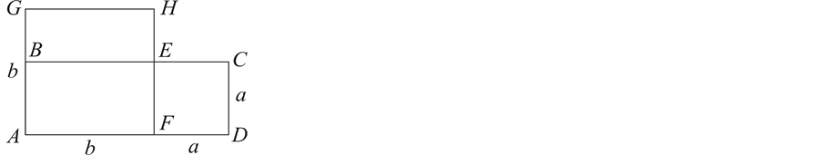
Figure 1. A division of a line segment in extreme and mean ratio (the “golden ratio”).

Figure 2. The golden ratio.
CB (Figure 2), that is,
 . (3)
. (3)
This is the definition of the “golden ratio,” used in modern science.
2.2. Algebraic Properties of the Golden Ratio
The following algebraic equation follows from the proportion (3):
 . (4)
. (4)
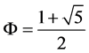
From the “physical meaning” of the proportion (3) implies that we should use the positive root of the equation (4). We denote this root through F:
 . (5)
. (5)
The following simple identities for
![]() follows from the algebraic equation:
follows from the algebraic equation:
 (6)
(6)
 . (7)
. (7)
 . (8)
. (8)
3. Fibonacci Numbers and Their Properties
Definition. The following recursive relation:
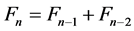 (9)
(9)
at the seeds
 (10)
(10)
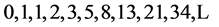
“generates” the following numerical sequence called Fibonacci numbers:
 (11)
(11)
The extended Fibonacci numbers. Fibonacci numbers have the following unique properties. First of all, Fibonacci numbers (11) can be extended to the negative values of n (Table 1).
The extended Fibonacci numbers are an infinite numerical sequence, which is determined
in the limits from
 to
to
 and has the following unique property:
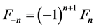 (12)
(12)
Cassini’ formula. The following identity, called Cassini’s formula, is valid for the arbitrary three adjacent Fibonacci numbers taken from Table 1:
 . (13)
4. Binet’s Formulas and Hyperbolic Fibonacci Functions
4.1. Binet’s Formulas
In 19 century, French mathematician Jacques Philippe Marie Binet (1776-1856) deduced the following formula, which connects the extended Fibonacci numbers and the golden ratio. In the book [24] these formulas are represented in the following non-traditional form:
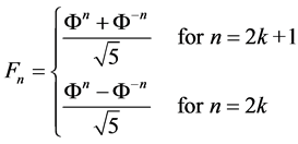 (14)
(14)
The analysis of the formula (14) gives us a possibility to feel “aesthetic pleasure”
and once again to be convinced in the beauty of mathematics! Really, we know that
the “extended” Fibonacci numbers (Table 1) always
are integers. On the other hand, any degree of the golden ratio is irrational number.
It follows from here that the integer numbers
 can be represented by using the formulas (14) through
the golden ratio
can be represented by using the formulas (14) through
the golden ratio
![]() and the irrational number
and the irrational number .
.
4.2. Hyperbolic Fibonacci Functions
A presentation of Binet’s formulas in the form (14) [24] has the following advantage. A comparison of Binet’s formulas (14) with the classic hyperbolic functions
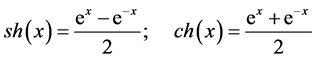 (15)
(15)
allows to see their similarity. Basing on this simple observation, the Ukrainian mathematicians Alexey Stakhov, Ivan Tkachenko and Boris Rozin came to the introduction of a new class of hyperbolic functions, called hyperbolic Fibonacci functions [14] -[17] :
Hyperbolic Fibonacci sine
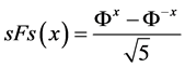 (16)
(16)
Hyperbolic Fibonacci cosine
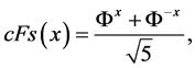 (17)
(17)

Table 1. The extended Fibonacci numbers.
Hyperbolic Fibonacci tangent
Hyperbolic Fibonacci cotangent
where x is continuous variable.
The uniqueness of the hyperbolic Fibonacci functions (16), (17) consists in the fact that they are inseparably related with the “extended” Fibonacci numbers. This relation follows from the comparison of hyperbolic Fibonacci functions (16), (17) with Binet’s formula (14) and can be represented as follows:
 (18)
(18)
where k takes the values from the set

This means that in the discrete points of the variable x
 the functions (16), (17) coincide with the extended Fibonacci numbers calculated
according to Binet’s formula (14).
the functions (16), (17) coincide with the extended Fibonacci numbers calculated
according to Binet’s formula (14).
Graphs of the hyperbolic Fibonacci functions. The above unique property of the functions (16), (17) is demonstrated in the best way on the graphs of the hyperbolic Fibonacci functions in Figure 3.
Here the graphs of the hyperbolic sine
 and the hyperbolic cosine
 are represented.
The “even” discrete points of the variable x
 on the graph
 correspond to the extended Fibonacci numbers with the even indexes
 , that is,
 . (19)
The “odd” discrete points of the variable x
 on the graph
 correspond to the extended Fibonacci numbers with the odd indexes
 , that is,
 (20)
(20)
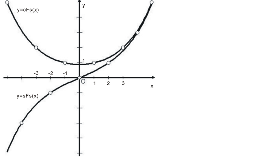
Figure 3. Hyperbolic fibonacci functions.
4.3. Comparison of the Hyperbolic Fibonacci Functions with the Classic Hyperbolic Functions
It is shown in [13] -[15]
, that the hyperbolic Fibonacci functions (16), (17) retain all hyperbolic properties
of the classic hyperbolic functions (15), however, these hyperbolic functions have
two new unique properties. Firstlythe “golden ratio”
 is the base of these functions and, secondly, they are deeply
connected, according to (18), with the extended Fibonacci numbers (see Table 1). This means that these functions are, on the one
hand, “harmonic” hyperbolic functions, based on the main “harmonic proportion” of
Nature (the “golden ratio”), and on the other hand, they have the recursive properties,
similarly to the extended Fibonacci numbers.
is the base of these functions and, secondly, they are deeply
connected, according to (18), with the extended Fibonacci numbers (see Table 1). This means that these functions are, on the one
hand, “harmonic” hyperbolic functions, based on the main “harmonic proportion” of
Nature (the “golden ratio”), and on the other hand, they have the recursive properties,
similarly to the extended Fibonacci numbers.
These unique properties of the hyperbolic Fibonacci functions (16), (17) are a confirmation of the fact that the hyperbolic Fibonacci functions (16), (17) are a fundamentally new class of hyperbolic functions, which are distinguished from the classic hyperbolic functions (15). The principal distinction of the hyperbolic Fibonacci functions (16), (17) from the classic hyperbolic functions (15) consists in the fact that they have recursive properties similarly to the extended Fibonacci numbers, which are a “discrete” analog of the functions (16) and (17) (see Figure 3). In the classic hyperbolic functions (15) such relationship with integer numerical sequences does not exist. This unique property of the new hyperbolic functions (16), (17) and its role in Nature has been confirmed recently by the new geometric theory of phyllotaxis, created by the Ukrainian researcher Oleg Bodnar [8] .
Taking into consideration the unique properties of the hyperbolic Fibonacci functions (16), (17), we have every right to say that the hyperbolic geometry, based on the classic hyperbolic functions (15), could develop in another way provided that Nikolay Lobachevski knew the functions (16), (17).
4.4. The Authority of Nature (Bodnar’s Geometry)
However, the new geometric theory of phyllotaxis, created by Ukrainian researcher Oleg Bodnar [8] -[11] , is the most powerful confirmation of the uniqueness of the hyperbolic Fibonacci functions. As is known, the appearance of the intersecting Fibonacci’s spirals on the surface of phyllotaxis objects is the main mystery of this wellknown botanical phenomenon.
Bodnar has studied growth’s problem of the phyllotaxis objects (pine cone, pineapple, cactus, sunflower’s head, etc.) and came to the unexpected conclusions. We will not describe in detail “Bodnar geometry”, referring the reader to Bodnar’ works [8] -[11] . We focus only on the key ideas of this geometry. Bodnar explores the growth of phyllotaxis objects and concludes that this growth is based on the notion of hyperbolic rotation, which is a key concept of hyperbolic geometry [25] .
However, the main idea of “Bodnar’s geometry” is to use the hyperbolic Fibonacci functions (16), (17) for the simulation of the growth of phyllotaxis objects. Using the hyperbolic Fibonacci functions (16), (17) for the description of all mathematical correlations of hyperbolic geometry, Oleg Bodnar obtained the special class of hyperbolic geometry, called “golden” hyperbolic geometry.
“Bodnar’s geometry” is distinguished substantially from Lobachevski’s geometry, based on the classic hyperbolic functions (15). This distinction consists in the fact that the main relations of this geometry are described in the terms of the hyperbolic Fibonacci functions (16) and (17), which are connected with the “extended” Fibonacci numbers by the simple relation (18).
The most important, that the unique mathematical relation (18) is the main cause of the Fibonacci spirals on the surface of phyllotaxis objects.
4.5. An Importance of the Hyperbolic Fibonacci Functions for Theoretical Natural Sciences
“Bodnar’s geometry” shows that the “phyllotaxis world” is a hyperbolic world based on the hyperbolic Fibonacci functions (16), (17). These functions are not “fiction” of mathematicians; they are “natural functions” that are used in natural objects during millions, maybe billions of years long before humanity’s appearance. That is why, the hyperbolic Fibonacci functions [14] -[17] , together with “Bodnar’s geometry” [8] -[11] can be attributed to the category of modern fundamental scientific discoveries, and in such quality they should remain in science. The vital importance of the hyperbolic Fibonacci functions (16), (17) for theoretical physics and theoretical natural sciences in the whole follows from the above reasoning.
5. Fibonacci (-Numbers as a Generalization of the Classical Fibonacci Numbers
5.1. Historical Information
In the late 20th and early 21st centuries, several researchers from different countries—Argentinean mathematician Vera W. de Spinadel [26] , French mathematician Midhat Gazale [27] , American mathematician Jay Kappraff [28] , Russian engineer Alexander Tatarenko [29] , Armenian philosopher and physicist Hrant Arakelyan [30] , Russian researcher Victor Shenyagin [31] , Ukrainian physicist Nikolai Kosinov [32] , Spanish mathematicians Falcon Sergio and Plaza Angel [33] and others independently one to another began to study a new class of recursive numerical sequences, which are a generalization of the classic Fibonacci numbers. These numerical sequences led to the discovery of a new class of mathematical constants, known as Spinadel’s “metallic means” [26] .
The interest of many independent researchers from different countries (USA, Canada, Argentina, France, Spain, Russia, Armenia, Ukraine) cannot be accidental. This means that the problem of the generalization of the Fibonacci numbers and “golden ratio” has matured in modern science.
5.2. A definition of the Fibonacci (-Numbers
Let us give a real number l > 0 and consider the following recurrence relation:
 (21)
(21)
with the seeds:
 (22)
(22)
The recurrence relation (21) with the seeds (22) generates an infinite number of new numerical sequences, because every real number l > 0 “generates” its own numerical sequence.
Let us consider the partial cases of the recurrence relation (21). For the case l = 1 the recurrence relation (21) and the seeds (22) are reduced to the following:
 (23)
(23)
 (24)
(24)
The recurrence relation (23) with the seeds (24) generates the classical Fibonacci numbers:
 . (25)
Based on this fact, we will name a general class of the numerical sequences, generated by the recurrence relation (21) with the seeds (22), the Fibonacci l-numbers.
For the case l = 2, the recurrence relation (21) and the seeds (22) are reduced to the following:
 ; (26)
 . (27)
The recurrence relation (26) with the seeds (27) generates the so-called Pell numbers [34] .
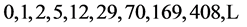 (28)
(28)
For the cases l = 3, 4 the recurrence relation (21) and the seeds (22) are reduced to the following:
 ;
; (29)
(29)
 ;
; . (30)
5.3. The “Extended” Fibonacci (-Numbers
The Fibonacci l-numbers have many remarkable properties, similar to the properties of the classical Fibonacci numbers. It easy to prove that the Fibonacci l-numbers, as well as the classical Fibonacci numbers, can be “extended” to the negative values of the discrete variable n.
Table 2 shows the four “extended” Fibonacci l-sequences, corresponding to the values l = 1, 2, 3, 4.
5.4. A Generalization of Cassini’s Formula
Cassini’s formula (13) for the classical Fibonacci numbers can be generalized for the case of the Fibonacci lnumbers. It is proved [35] that the generalized Cassini formula has the following form:
 (31)
(31)
Consider the example of the validity of the identity (31) for the the
 -sequence for the case of n = 7. For this case we should
consider the following triple of the Fibonacci 2-numbers
-sequence for the case of n = 7. For this case we should
consider the following triple of the Fibonacci 2-numbers :
:
 .
.
By performing the calculations over them according to (31), we get the following result:
 what corresponds to the identity (31), because for the
case n = 7 we have:
what corresponds to the identity (31), because for the
case n = 7 we have:
 .
.
Thus, by studying the generalized Cassini formula (31) for the Fibonacci l-numbers,
we came to the discovery of an infinite number of integer recurrence sequences in
the range from
 to
to , with the following unique mathematical property (31),
which sounds as follows:
, with the following unique mathematical property (31),
which sounds as follows:
The quadrate of any Fibonacci (-number
 are always different from the product of the two adjacent Fibonacci (-numbers
 and
and , which surround the initial Fibonacci (-number
 , by the number 1; herewith the sign
of the difference of 1 depends on the parity of n: if n is even, then the difference
of 1 is taken with the sign “minus,” otherwise, with the sign “plus.”
, by the number 1; herewith the sign
of the difference of 1 depends on the parity of n: if n is even, then the difference
of 1 is taken with the sign “minus,” otherwise, with the sign “plus.”
Until now, we have assumed that only the classical Fibonacci numbers have the similar unusual property, given by Cassini’s formula (13). However, as is proved in [35] , a number of such numerical sequences are infinite. All the Fibonacci l-numbers, generated by the recurrence relation (21) with the seeds (22), have a similar property, given by the generalized Cassini’s formula (31)!
As is well known, a study of integer sequences is the area of number theory. The
Fibonacci l-numbers are integers for the cases . Therefore, for many mathematicians
in the field of number theory, the existence of the infinite number of the integer
sequences, which satisfy to the generalized Cassini’s formula (31), may be a big
surprise.
. Therefore, for many mathematicians
in the field of number theory, the existence of the infinite number of the integer
sequences, which satisfy to the generalized Cassini’s formula (31), may be a big
surprise.
6. The “Metallic Means”
6.1. The Algebraic Equation for the Fibonacci (-Numbers
Let us represent the recurrence relation (21) as follows:
Table 2. The “extended” Fibonacci l-numbers (l = 1, 2, 3, 4).
 (32)
(32)
For the case , the expression (32) is reduced to the
following quadratic equation:
, the expression (32) is reduced to the
following quadratic equation:
 . (33)
with the roots
 and
and .
(34)
.
(34)
6.2. The “Metallic Means” by Vera de Spinadel
Denote the positive root x1 of the equation (33) by , that is,
 (35)
(35)
Note that for the case
![]() the formula (35) is reduced to the formula for the “golden ratio”:
the formula (35) is reduced to the formula for the “golden ratio”:
 . (36)
This means that formula (35) is a generalization of the “golden ratio” and expresses a new class of mathematical constants.
Basing on this reasoning, the Argentinean mathematician Vera de Spinadel [26] named the mathematical constants (35) metallic means. If we take l = 1, 2, 3, 4 in (35), then we get the following mathematical constants, having, according to Vera de Spinadel, special names:
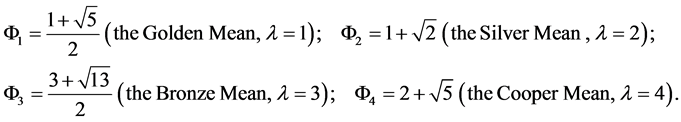
Other metallic means
 do not have special names:

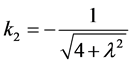
It is easy to prove that the root x2 (34) can be represented through the metallic mean (35) as follows:
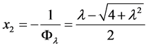 . (37)
Also it is easy to prove the following identity:
 , (38)
where n = 0, ±1, ±2, ±3,
6.3. Two Surprising Representations of the “Metallic Means”
For the case n = 2, the identity (38) can be represented in the form:
 (39)
(39)
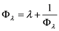
It follows from (39) the following representation of the “metallic mean”:
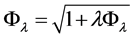 (40)
(40)
Substituting
 instead
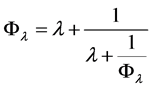
 in the right-hand part of (40) we get:
 (41)
(41)
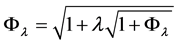
Continuing this process ad infinitum, that is, substituting repeatedly
 instead
 in the righthand part of (41), we get the following surprising representation of
the “metallic mean”
in the righthand part of (41), we get the following surprising representation of
the “metallic mean”
 in “radicals”:
 (42)
(42)
Represent now the identity (39) in the form:
 (43)
(43)
Substituting
 instead
 in the right-hand part of (43), we get:
 (44)
(44)
Continuing this process ad infinitum, that is, substituting
 repeatedly instead
 in the right-hand part of (44), we get the following surprising representation of
the “metallic mean”
in the right-hand part of (44), we get the following surprising representation of
the “metallic mean”
 in the form of “continued fraction”:
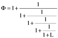
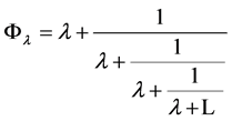 (45)
(45)
Note that for the case
![]() the representations (42) and (45) coincide with the well known representations of
the classical golden ratio, given by the expressions (7), (8).
the representations (42) and (45) coincide with the well known representations of
the classical golden ratio, given by the expressions (7), (8).
7. Gazale’s Formula and Hyperbolic Fibonacci (-Functions
7.1. Gazale’s Aormula
The formulas (21), (22) define the Fibonacci l-numbers
 by recursion. We can represent the numbers
 in the explicit form through the “metallic mean”
 .
.
With this purpose, we can represent the Fibonacci l-numbers
 by the roots x1 and x2 in the form:
 , (46)
where k1 and k2 are constant coefficients, which are the solutions of the following system of algebraic equation:
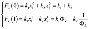 (47)
(47)
Taking into consideration that
 and
and , we can rewrite the system (47) as follows:
 (48)
(48)
Taking into consideration (48), we can find the following formulas for the coefficients k1 and k2:
 ;
; (49)
(49)
Taking into consideration (49), we can rewrite the formula (46) as follows:
 (50)
(50)
Taking into consideration that
 and
and , we can rewrite the formula (50) as follows:
 (51)
(51)
or
 (52)
(52)
After simple transformations formula (52) can be represented as follows:
 , (53)
where .
.
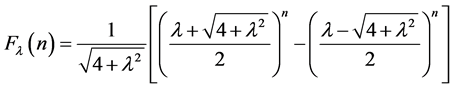
Note that the formula (51) was first obtained by the French mathematician Midhat
Gazale [27] . A distinctive feature of Gazale’s
formulas (53) is the fact that they include an infinite number of the formulas (53),
because each real number
![]() “generates” its own Gazale’s formula (53). In particular, for the case l = 1 Gazale’s
formula (53) are reduced to Binet’s formula (13).
“generates” its own Gazale’s formula (53). In particular, for the case l = 1 Gazale’s
formula (53) are reduced to Binet’s formula (13).
7.2. Hyperbolic Fibonacci (-Functions
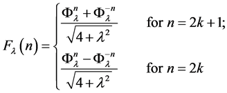
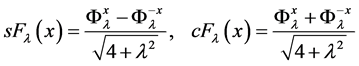
Gazale’s formula (53) led to the introduction of the new class of hyperbolic functions called hyperbolic Fibonacci l-functions [18] [19] :
Hyperbolic Fibonacci l-sine
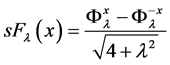 (54)
(54)
Hyperbolic Fibonacci l-cosine
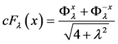 , (55)
Hyperbolic Fibonacci l-tangent
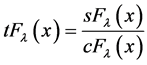
Hyperbolic Fibonacci cotangent

where l > 0 is a given real number,
 is “metallic proportion.”
The hyperbolic Fibonacci l-functions (54), (55) have a number of unique mathematical properties.
First of all, we note that a number of the hyperbolic Fibonacci l-functions (54), (55) are infinite theoretically, because every real number l > 0 “generates” its own class of the functions (54), (55). Note that for the case l = 1, the functions (54), (55) are reduced to the hyperbolic Fibonacci functions (16), (17), introduced in [15] -[17] .
The uniqueness of the hyperbolic Fibonacci l-functions. It follows from the comparison
of Gazale’s formula (53) and hyperbolic Fibonacci l-functions (54), (55) that the
hyperbolic Fibonacci l-functions (54), (55) coincide with the extended Fibonacci
l-numbers (see Table 2) in the discrete points
of the variable
 , that is,
 . (56)
The formula (56) determines the uniqueness of the hyperbolic Fibonacci l-functions.
The formula (56) means that in the “even” discrete points of the variable x
 the hyperbolic Fibonacci l-functions coincide with the “extended” Fibonacci l-numbers
with the even indexes
the hyperbolic Fibonacci l-functions coincide with the “extended” Fibonacci l-numbers
with the even indexes , that is,
 (57)
(57)
In the “odd” discrete points of the variable x
 the hyperbolic Fibonacci l-functions coincide with the “extended” Fibonacci l-numbers
with the odd indexes
the hyperbolic Fibonacci l-functions coincide with the “extended” Fibonacci l-numbers
with the odd indexes![]() , that is,
, that is,
 . (58)
8. Euclid’s Fifth Postulate and Lobachevski’s Geometry
On February 23, 1826 on the meeting of the Mathematics and Physics Faculty of Kazan University the Russian mathematician Nikolai Lobachevski (1792-1856) had proclaimed on the creation of new geometry named imaginary geometry. This geometry was based on the traditional Euclid’s postulates, excepting Euclid’s Fifth Postulate about parallels. New Fifth Postulate about parallels was formulated by Lobachevski as follows: “At the plane through a point outside a given straight line, we can conduct two and only two straight lines parallel to this line, as well as an endless set of straight lines, which do not overlap with this line and are not parallel to this line, and the endless set of straight lines, intersecting the given straight line.”
For the first time, a new geometry was published by Lobachevski in 1829 in the article About the Foundations of Geometry in the magazine Kazan Bulletin.
Independently on Lobachevski, the Hungarian mathematician Janos Bolyai (1802-1860) came to such ideas. He published his work Appendix three years later Lobachevski (1832). Also the prominent German mathematician Carl Friedrich Gauss (1777-1855) came to the same ideas. After his death some unpublished sketches on the non-Euclidean geometry were found.
Lobachevski’s geometry got a full recognition and wide distribution 12 years after his death, when it is became clear that scientific theory, built on the basis of a system of axioms, is considered to be fully completed only when the system of axioms meets three conditions: independence, consistency and completeness. Lobachevski’s geometry satisfies these conditions. Finally this became clear in 1868 when the Italian mathematician Eugenio Beltrami (1835-1900) in his memoirs The Experience of the Non-Euclidean Geometry Interpretation showed that in Euclidean space at pseudo-spherical surfaces geometry of Lobachevski’s plane arises, if we take geodesic lines as straight lines.
Later the German mathematician Felix Christian Klein (1849-1925) and the French mathematician Henri Poincare (1854-1912) proved a consistency of Non-Euclidean geometry, by means of the construction of corresponding models of Lobachevski’s plane. The interpretation of Lobachevski’s geometry on the surfaces of Euclidean space contributed to general recognition of Lobachevski’s ideas.
The creation of Riemannian geometry Georg Friedrich Bernhard Riemann (1826-1866), became the main outcome of such Non-Euclidean approach. The Riemannian geometry developed a mathematical doctrine about geometric space, a notion of differential of a distance between elements of diversity and a doctrine about curvature.
The introduction of the generalized Riemannian spaces, whose particular cases are Euclidean space and Lobachevski’s space, and the so-called Riemannian geometry, opened new ways in the development of geometry. They found their applications in physics (theory of relativity) and other branches of theoretical natural sciences.
Lobachevski’s geometry also is called hyperbolic geometry because it is based on the hyperbolic functions (15), introduced in 18th century by the Italian mathematician Vincenzo Riccati (1707-1775).
The most famous classical interpretations of Lobachevski’s plane with the Gaussian curvature K < 0, are the following:
-Beltrami’s interpretation on a disk;
-Poincare’s interpretation on a disk.
-Klein’s interpretation at a half-plane and other.
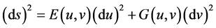
Lobachevsky metric is called the metric form
 (59)
(59)
with the Gaussian curvature , where the variables (u, v) belong to
the half-plane
, where the variables (u, v) belong to
the half-plane
![]() . (60)
. (60)
Here ds is called an arc length and
 is hyperbolic sine.
Lobachevsky’s geometry has remarkable applications in many fields of modern natural sciences. This concerns not only applied aspects (cosmology, electrodynamics, plasma theory), but, first of all, it concerns the most fundamental sciences and their foundation, mathematics (number theory, theory of automorphic functions created by A. Poincare, geometry of surfaces and so on).
Since on the closed surfaces of the negative Gaussian curvature, Lobachevski’s geometry is fulfilled and Lobachevski’s plane is universal covering for these surfaces, it is very fruitful to study various objects (dynamical systems with continuous and discrete time, layers, fabrics and so on), defined on these surfaces. By developing this idea, we can raise these objects to the level of universal covering, which is replenished by the absolute (“infinity”), and further we can study smooth topological properties of these objects with the help of the absolute.
Samuil Aranson studied this problem about four decades. The works [36] -[41] , written by Samuil Aranson with co-authors, give a presentation about these results and research methods. Aranson’s DrSci dissertation “Global problems of qualitative theory of dynamic systems on surfaces” (1990) is devoted to this theme.
9. Hilbert’s Fourth Problem
9.1. A brief History
In the lecture “Mathematical Problems” [42] , presented at the Second International Congress of Mathematicians (Paris, 1900), David Hilbert (1862-1943) had formulated his famous 23 mathematical problems. These problems determined considerably the development of the 20th century mathematics. This lecture is a unique phenomenon in the mathematics history and in mathematical literature.
The Russian translation of Hilbert’s lecture and its comments are given in the book [42] . In Hilbert’s original work [43] Hilbert’s Fourth Problem is called as follows: “Problem of the straight line as the shortest distance between two points.” In [43] this problem was formulated as follows:
“Another problem relating to the foundations of geometry is this: If from among the axioms necessary to establish ordinary euclidean geometry, we exclude the axiom of parallels, or assume it as not satisfied, but retain all other axioms, we obtain, as is well known, the geometry of Lobachevsky (hyperbolic geometry). We may therefore say that this is a geometry standing next to euclidean geometry…
The more general question now arises: Whether from other suggestive standpoints geometries may not be devised which, with equal right, stand next to Euclidean geometry”…
The theorem of the straight line as the shortest distance between two points and the essentially equivalent theorem of Euclid about the sides of a triangle, play an important part not only in number theory but also in the theory of surfaces and in the calculus of variations. For this reason, and because I believe that the thorough investigation of the conditions for the validity of this theorem will throw a new light upon the idea of distance, as well as upon other elementary ideas, e.g., upon the idea of the plane, and the possibility of its definition by means of the idea of the straight line, the construction and systematic treatment of the geometries here possible seem to me desirable.”
Hilbert’s citations contain the formulation of very important mathematical problems, which touch foundation of geometry, number theory, the theory of surfaces and the calculus of variations. Hilbert’s Fourth Problem is of fundamental interest not only for mathematics, but also for all theoretical natural sciences: are there non-Euclidean geometries, which are next to Euclidean geometry and are interesting from the “other suggestive standpoints? If we consider it in the context of theoretical natural sciences, then Hilbert’s Fourth Problem is about finding NEW HYPERBOLIC WORLDS OF NATURE, which are next to Euclidean geometry and reflect some new properties of Nature’s structures and phenomena.
Note that Hilbert considered Lobachevski’s geometry and Riemann’s geometry as nearest to Euclidean geometry. As it is noted in Wikipedia [44] , “in mathematics, Hilbert’s Fourth Problem in the 1900 ‘Hilbert problems’ was a foundational question in geometry. In one statement derived from the original, it was to find geometries whose axioms are closest to those of Euclidean geometry if the ordering and incidence axioms are retained, the congruence axioms weakened, and the equivalent of the parallel postulate omitted.”
In mathematical literature Hilbert’s Fourth Problem is sometimes considered as formulated very vague what makes difficult its final solution. As it is noted in Wikipedia [44] , “the original statement of Hilbert, however, has also been judged too vague to admit a definitive answer.” In [45] American geometer Herbert Busemann analyzed the whole range of issues related to Hilbert’s Fourth Problem and also concluded that the question related to this issue, unnecessarily broad.
Unfortunately, the attempts solving Hilbert’s Fourth Problem, made by German mathematician Herbert Hamel (1901) and later by Soviet mathematician Alexey Pogorelov [46] (1974), have not led to significant progress, as pointed out in Wikipedia’s articles [43] [44] . In order to learn more about an axiomatic approach to solving the Hilbert’s Fourth Problem by wonderful geometer A.V. Pogorelov, see also Aranson’s article [47] .
In Wikipedia’s article [43] , the status of the problem is formulated as “too vague to be stated resolved or not” and Pogorelov’s book [46] even is not mentioned.
About the same point of view on Hilbert’s Fourth Problem is presented in the remarkable book [48] . Unfortunately, this important problem is still not resolved. Currently, most mathematicians are inclined to believe that Hilbert’s Fourth Problem has been formulated too vague what makes complicated its final solution. That is, the mathematicians of the 20th century laid the blame for the failure in the solution of this problem on Hilbert himself.
In spite of critical attitude of mathematicians to Hilbert’s Fourth Problem, we should emphasize a great importance of this problem for mathematics, particularly for geometry. Without doubts, Hilbert's intuition led him to the conclusion that Lobachevski’s geometry and Riemann’s geometry do not exhaust all possible variants of non-Euclidean geometries. Hilbert’s Fourth Problem directs researchers at finding new non-Euclidean geometries, which are the nearest geometries to the traditional Euclidean geometry.
9.2. From the “Game of Postulates” to the “Game of Functions”
According to [49] , a cause of difficulty in the solution of Hilbert’s Fourth Problem lies elsewhere. All the known attempts to solve this problem (Herbert Hamel, Alexey Pogorelov) were in the traditional framework of the socalled “game of postulates” [49] .
This “game” started from the works by Nikolai Lobachevski and Janos Bolyai, when Euclid’s 5th postulate was replaced by the opposite one. This was the most major step in the development of the non-Euclidean geometry, which led to “Lobachevski’s geometry.” This geometry, which changed the traditional geometric representations, is also known as “hyperbolic geometry.” This name highlights the fact that this geometry is based on the classical hyperbolic functions (15). And this is the main idea of “Lobachevski’s geometry.”
It is important to emphasize that the very name of “hyperbolic geometry” points on another approach to the solution of Hilbert’s Fourth Problem: searching for the new classes of “hyperbolic functions,” which can be the basis for other hyperbolic geometries. As is shown above, the general theory of “harmonic” hyperbolic functions, based on the “golden” and “metallic” proportions, was developed recently [14] -[19] . Every new class of the “harmonic” hyperbolic functions (16), (17), generates its own new variant of the “hyperbolic geometry.” By analogy with the “game of postulates” this approach solving Hilbert’s Fourth Problem can be named the “game of functions” [49] .
10. Basic Notions and Concepts
10.1. Preliminary Information
Lobachevski’s metric form (59) can be obtained (see e.g. [50] ) when considering of the upper half of the twosheeted hyperboloid (pseudo-sphere of the “radius” R):

![]() , (61)
, (61)
embedded in three-dimensional pseudo-Euclidean space (X, Y, Z) with Minkowski’s metrics
 .
.
Here dl is the arc element in the space (X, Y, Z), with the next parameterization of the surface (60) in the form:
![]() , (62)
, (62)
where the half-plane (60)
![]() is the domain of existence of curvilinear coordinates (u, v).
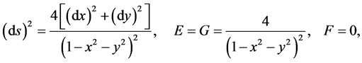
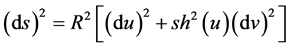
With this parameterization of М2 for the metric (59) we have:
is the domain of existence of curvilinear coordinates (u, v).
With this parameterization of М2 for the metric (59) we have: .
.
In the special theory of relativity (STR) we use the following coordinate system:
the spatial coordinates X, Y, the time coordinate , where
 is the light velocity in vacuum, t is a time. Figure 4
gives a visual representation of the surface
is the light velocity in vacuum, t is a time. Figure 4
gives a visual representation of the surface . The surface
 belongs to the so-called time-homothetic domain, bounded by the upper half of the
isotropic (in other terminology, light) cone K2:
belongs to the so-called time-homothetic domain, bounded by the upper half of the
isotropic (in other terminology, light) cone K2: , Z > 0.
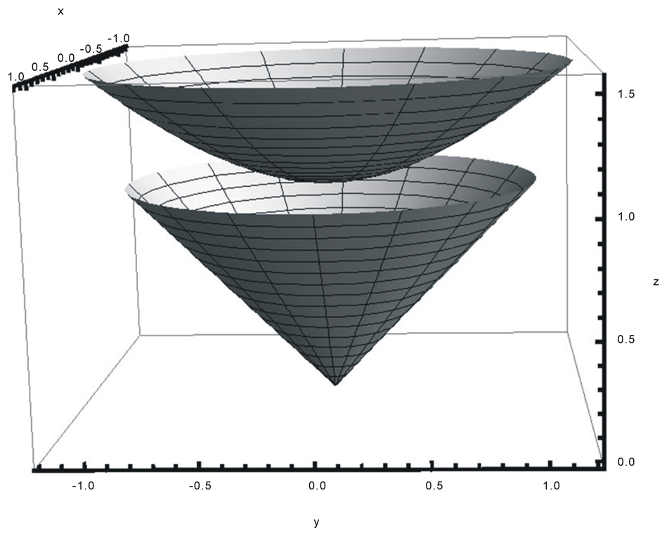
Figure 4. The surface M2.
Note that the surface
 is considered as the upper half of two-sheeted hyperboloid, embedded into Minkowski’s
three-dimensional space. From this point of view the surface
is considered as the upper half of two-sheeted hyperboloid, embedded into Minkowski’s
three-dimensional space. From this point of view the surface
 is considered as an open two-dimensional manifold. All the considered below parametric
representation of this surface in those or other curvilinear coordinates are nothing
as covering of the manifold
is considered as an open two-dimensional manifold. All the considered below parametric
representation of this surface in those or other curvilinear coordinates are nothing
as covering of the manifold
 by the different sets of the cards
 with recalculation from one card to another card, while in this situation, each
such card completely covers all the two-dimensional manifolds
with recalculation from one card to another card, while in this situation, each
such card completely covers all the two-dimensional manifolds .
.
In further, each card will have an independent life in isolation from the surface
 as interpretation of those or other Lobachevski’s models with specifically introduced
metrics (the Lobachevski’s plane with Lobachevski’s metric, Poincare’s model on
the disk, Klein’s model on the half-plane, an infinite set of models of the authors
of this article, which preserve invariance of half-plane.
as interpretation of those or other Lobachevski’s models with specifically introduced
metrics (the Lobachevski’s plane with Lobachevski’s metric, Poincare’s model on
the disk, Klein’s model on the half-plane, an infinite set of models of the authors
of this article, which preserve invariance of half-plane.
Each such model with specifically introduced metric has its own individual unique geometric and differential properties and requires of separate investigation.
At the same time when we convert one model into another model, these properties are interpreted differently. In this case, the following questions appear: whether the Gaussian curvature remains constant, how geodesic lines, angles, squares of figures in a particular model are changing, what are movements, compressions, conversions, which are not movements, how we should study dynamical systems, as the one-parameter groups of transformations with continuous and discrete time and so on. In this case, a study of the absolute arithmetic properties for such models, for the limiting continuation of such transformations on the absolute, are important from theoretical and practical point of view.
Of particular interest is the study of such models as the universal ramified or
non-ramified covering spaces
 , when we present the closed orientable and non-orientable
surface M of Euler’s negative characteristic
, when we present the closed orientable and non-orientable
surface M of Euler’s negative characteristic
 in the form of factor
 of the covering spaces
 for the discrete groups of the transformations G.
10.2. The Notion of the Absolute
In our study, the important role plays the concept of the absolute, replenishing
the space . These issues are studied in many works of
the second author Samuil Aranson (see, for example, in the monographs [36] -[41]
[51] ).
. These issues are studied in many works of
the second author Samuil Aranson (see, for example, in the monographs [36] -[41]
[51] ).
In order to introduce the concept of the absolute for the following non-Euclidean metric forms, we pre-equip the entire plane or three-dimensional space with Euclidean metric.
Then we further equip with the non-Euclidean metric form a certain area of the Euclidean
plane or a surface in three-dimensional Euclidean space. We will call the absolute
of non-Euclidean metric form the boundary
![]() of the domain of definition D of this form, such that at approaching to
of the domain of definition D of this form, such that at approaching to
![]() “inside” of the domain D, the non-Euclidean form degenerates.
“inside” of the domain D, the non-Euclidean form degenerates.
Below we consider three non-Euclidean metric forms of the Gaussian curvature![]() , which are the interpretation of Lobachevski’s geometry.
, which are the interpretation of Lobachevski’s geometry.
1). For Poincare’s metric form
given on the disc
 of the Euclidean plane
 , the absolute is the so-called “infinity circle”
 .
.
At approaching “from within” the area
 along of any ray to the “infinity circle”
 we get:
 that is, Poincare’s metric form degenerates.
2). For Lobachevski’s metric form
 given on the half-plane
 of the Euclidean plane
 , the absolute
![]() has the following form:
has the following form:
 where
where
 -v is the axis of the Euclidean plane
 ,
,
 is an “infinitely distant line.”
At approaching “from within” the area
 along of any ray to the
 -axis
-axis
 we get:
![]() and hence Lobachevski’s metric form degenerates.
and hence Lobachevski’s metric form degenerates.
A similar situation is obtained also at approaching “from within” the area
 along of any ray to an “infinitely distant line”
 , since then
![]() that is, Lobachevski’s metric form again degenerates.
that is, Lobachevski’s metric form again degenerates.
3). For Minkovski’s metric form
 given on the pseudo sphere
 in the Euclidean space
 , here the absolute is the “infinitely distant
circumference”
, here the absolute is the “infinitely distant
circumference” , which “belongs” to the upper half
 of the light cone
 .
.
Proof. According to [50], the pseudo
sphere
 admits a parametrization

where

is Poincare’s metric form on the disc .
.
It follows from the above Poincare’s metric form, that the absolute is a circumference
 and because
 then at approaching
 “from within” the area
 , we get
 .
.
This means that the “infinitely distant circumference”
 is the absolute for Minkovski’s metric form.
10.3. Two-Parametric Family of Linear Transformations
Let us pass to the specific results, obtained by the authors and related to Hilbert’s Fourth Problem, and their interpretation by using the notions of the “golden ratio” and “metallic proportions” [26] .
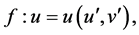
By direct computation, it is easy to find that the surface
 given (61) is also invariant at the parametrization
 , (63)
where
 are smooth functions,
However, for such arbitrary parametrization, the certain geometric structures and
differential properties at one-to-one mapping of the surface
 can be violated, a priori.
Here and below (unless otherwise stated) we restrict ourselves by the two-parametric
family of linear transformations (63) of the half-plane , for the conditions, when the change of variables
 according to the transformation (63) into the variables
 are fulfilled by the rule:
 (64)
(64)
where
 are some real numbers satisfying to the conditions:
 (65)
(65)
Thus, in this situation, the transformation (64) is the introduction of new coordinates
in the half-plane , such, when the new coordinates
 everywhere in the half-plane П+ can be expressed through the old coordinates
and vice versa. From the viewpoint of Riemannian geometry, the twoparametric transformation
(64) has their special specific properties.
everywhere in the half-plane П+ can be expressed through the old coordinates
and vice versa. From the viewpoint of Riemannian geometry, the twoparametric transformation
(64) has their special specific properties.
Further on the half-plane П+ for any fixed positive value of R > 0 we will compare (unless otherwise stated), two metric forms of the kind:
1). Lobachevski’s metric form
 , (66)
2). Two-parametric metric form
 (67)
(67)
The metric form (66) is converted into the form (67) under the action of diffeomorphism
(64) for each value of the real numbers , satisfying to the condition (65).
Here
 are elements of arc lengths,
 -coefficients of metric forms.
Metric forms in terms of tensor analysis are symmetric covariant tensor field of the rank two on a smooth manifold. Through this manifold, the scalar product on the tangent space, the length of curves, angles between curves, squares and so on are given.
To identify the specific properties of the transformations (64) and their effect on the metric forms, pre-recall some basic concepts, related to the nonsingular quadratic metric forms of internal geometry and their transformations induced by diffeomorphisms (see, for example, [50] [52] ).
10.4. Isometric Mapping and Equivalence, Isometry, and Conformal Metric Forms
First of all, we will make some changes in some definitions and concepts, because different sources give different interpretations of these concepts.
Suppose further that, unless otherwise stated, we consider the half-plane
 ,
,
where three objects are given:
1). Diffeomorphism
 . (68)
2). Metric form
 , (69)
where the coefficients satisfy to the non-equalities:
3). Metric form
 , (70)
where the coefficients satisfy to the non-equalities: .
.
Definition 1. We say that the diffeomorphism (68) is an isometric map if under the influence of this diffeomorphism the metric form (69) is converted to the metric form (70), while the lengths of the elements satisfy the condition:
 . (71)
The metric forms (69) and (70), satisfying to the condition (71) is called isometrically equivalent.
Thus, under the action of isometric mapping, the elements of arc lengths remain
the same, although the metric forms in the variables
 and
and
 may have different forms, and therefore may not preserve the same angles between
the arcs.
may have different forms, and therefore may not preserve the same angles between
the arcs.
Under the effect of the isometric mapping (68), the metric form (69) is converted into the metric form (70) of the following form:
![]()
![]() , (72)
, (72)
where
 (73)
(73)
Definition 2. We say that the diffeomorphism (68) is an isometry, if under the action
of the diffeomorphism (68) the metric form (69) is converted into the metric form
(70) for the variables
 having the same form as the metric form (69) for the variables
 , that is, for the case of the isometry the coefficients
of the metrical forms (70) and (69) satisfy to the following identities:
, that is, for the case of the isometry the coefficients
of the metrical forms (70) and (69) satisfy to the following identities:
 (74)
(74)
The metric forms (69) and (70), satisfying to the condition (74), is called isometrically identical. Diffeomorphisms, which are isometries, retain the same values of arc lengths and angles between the arcs.
Note that identical isometric metric forms are also automatically isometrically equivalent, the converse is not always true.
Definition 3. Diffeomorphism (68) is called conformal (angles between the arcs remain the same), and (69) and (70) are called conformal metric forms, if under the action of the diffeomorphism (68)
 , the metric form (69)
 differs from the metric form (70)
 by the positive factor
 .
.
In this case, the metric form (70), under the action of the diffeomorphism
 , is converted to the metric form
 , (75)
with the following coefficients:
![]() (76)
(76)
what corresponds to the following identities:
 (77)
(77)
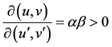
Definition 4. Mapping f:
 ,
,
 is called equireal (saves areas), if
 . (78)
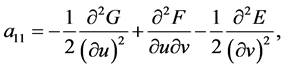
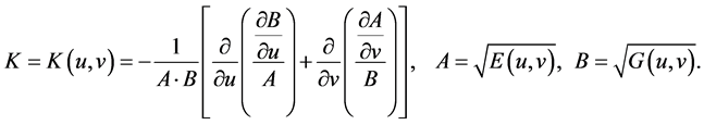
10.5. Gaussian Curvature
Gaussian curvature as a measure of the deformation of the surface is another important
notion of the internal geometry. We will not give a precise definition of this notion
(more in detailed see [50] [52] ). We only note thatif we know the metric form , then the Gaussian curvature
 is calculated by the formula:
 , (79)
where

 ,
,
 ,
,
 ,
,
 ,
,
 ,
,
 ,
,
 ,
,
 ,
,
 ,
,
 ,
,
 ,
,
 ,
,
 ,
,
 ,
,
 ,
,
 ,
, .
.
In our situation, we consider the metric forms, for which we have: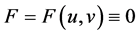 , and then, according to this remark, we get
from (79) the following formula for the Gaussian curvature:
, and then, according to this remark, we get
from (79) the following formula for the Gaussian curvature:
 (80)
(80)
10.6. A notion of the Distance
Let us introduce the concept of the distance
 between Lobachevski’s metric form (66) and two-parametric metric form (67)
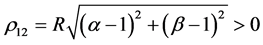
Definition 5. The following number:
 (81)
(81)
is called the distance between Lobachevski’s metric form (66)
 and the two-parametric metric form (67)
 , where
 ,
,![]() .
.
Note that for the case
 we have
 , and then the metric forms (66) and (67) have
the same form, and therefore they are isometrically identical, here the isometry
has the following form:
, and then the metric forms (66) and (67) have
the same form, and therefore they are isometrically identical, here the isometry
has the following form: .
.
For brevity, we will say that for the case
 the metric form (67) coincides with Lobachevski’s metric form (66). For the case
 , the metric form (67) does not coincide with Lobachevski’s
metric form (66). In this case, either both numbers
, the metric form (67) does not coincide with Lobachevski’s
metric form (66). In this case, either both numbers
 is not equal to 1, or one of these numbers is equal to 1 and another number is not
equal to 1.
is not equal to 1, or one of these numbers is equal to 1 and another number is not
equal to 1.
We say that the metric form (67) is
 -close to Lobachevski’s metric form (66), if for any
![]() there is
there is
 such that for all
 the inequality
 exists.
Further, for the case
 we compare Lobachevski’s metric form (66) and the two-parametric form (67), obtained
from (66) under the action of the transformation (64), for compatibility or incompatibility
of the following properties of the interior geometry: Gaussian curvature, isometric
equivalence, isometric identity, conformity, conservation of areas.
we compare Lobachevski’s metric form (66) and the two-parametric form (67), obtained
from (66) under the action of the transformation (64), for compatibility or incompatibility
of the following properties of the interior geometry: Gaussian curvature, isometric
equivalence, isometric identity, conformity, conservation of areas.
10.7. Verifications
Verification to match the Gaussian curvature for the case (12 > 0
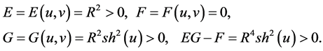
1) Lobachevski’s metric form (66):
 ,
,
![]()
![]()

 .
.
The Gaussian curvature of Lobachevski’s metric form is:
 (82)
(82)
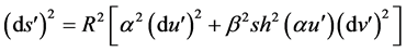
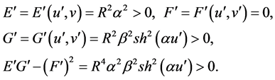
2) Two-parametric metric form (67), induced by the action of the transformation (64) on Lobachevski’s metric form (66).
Here the induced two-parametric metric form (67) has the following form:
 ,
,
![]() .
.
 ,
,
![]() ,
,
 ,
, .
.
The Gaussian curvature of the two-parametric metric form is the following:
 .
.
Conclusion. For the case
 the Gaussian curvature of the two-parametric metric form (67) for any
 coincides with the Gaussian curvature of Lobachevski’s metric form (66) and equal

Verification on isometric equivalence for the case (12 > 0
1) Lobachevski’s metric form (66)

![]()
2) Two-parametric metric form (67), induced by the action of the transformation (64) on Lobachevski’s metric form (66):
 ,
,

 ,
,
 ,
,
 ,
,

 ,
,
![]() ,
,
 ,
,
![]()
We verify the feasibility of the identities (5.14) on isometric equivalence:
For the case
 the formula (82) takes the following form:

From here, we get the following identities:
 ,
,
 ,
,
![]()
Conclusions. For the case
 the transformations (64)
 of the half-plane
 are isometric mapping, here Lobachevski’s metric form (66) and the two-parametric
metric forms (67), under the action of this transformation on (66), are isometrically
equivalent for any
are isometric mapping, here Lobachevski’s metric form (66) and the two-parametric
metric forms (67), under the action of this transformation on (66), are isometrically
equivalent for any
 such that either both numbers
 is not equal to 1, or one of these numbers equals to 1 and another number not equals
to 1.
is not equal to 1, or one of these numbers equals to 1 and another number not equals
to 1.
Verification on isometric identity for the case (12 > 0
1) Lobachevski’s metric form (66):

![]()
2) Two-parametric metric form (67), induced by the action of the transformation (64) on Lobachevski’s metric form (66), has the following form:
 ,
,

 ,
,
![]() .
.
In virtue of the Definition 2, in order that the mapping , was an isometry, the following identities should
be fulfilled:
, was an isometry, the following identities should
be fulfilled:
 where
where

 .
.
For the case
 and the assumption about the isometry, we get:
![]() , (83)
, (83)

![]() (84)
(84)
Since from the first identity (83) we have that![]() , then the mapping f takes the following form:
, then the mapping f takes the following form: . Hence,
 , but because u > 0 , then from the identity (84) we get:

So, we get that![]() ,
,
 , whence we have:
 what contradicts to the condition:

Conclusions. For the case , the transformation (64)

 of the half-plane
 at the condition (65)
 is not isometry, here Lobachevski’s metric form (66) and the
two-parametric metric forms (67) under the action of this transformation on (66)
are not identical isometrically.
is not isometry, here Lobachevski’s metric form (66) and the
two-parametric metric forms (67) under the action of this transformation on (66)
are not identical isometrically.
Verification on conformity for the case
 и
и ,
,

1) Lobachevski’s metric form (66):

![]()
2) Two-parametric metric form (67), induced by the action of the transformation (64) on Lobachevski’s metric form (66), has the following form:
 ,
,

 ,
,
![]() .
.
In virtue of the Definition 3, in order that the mapping
 was conformal, the following identities should be fulfilled:
![]()
where

 , and
, and
 is some function (the coefficient of conformality).
For the case
 and the assumption about the conformality, we get:
![]() , (85)
, (85)
![]() ,
,
![]() . (86)
. (86)
In virtue of the first identity (85), we have , therefore the mapping f takes the following
form: f:
, therefore the mapping f takes the following
form: f: ,
, . Hence, from the identity (86) and the condition
 , we get:

But then we have:
 what contradicts to the conditions

 .
.
Conclusions. For the case ,
,
 the transformations (64)
 of the half-plane
 for the condition (65)
 are not conformal, аnd the metric forms (66) and (67), under
the action of this transformation, are not conformal metric forms.
are not conformal, аnd the metric forms (66) and (67), under
the action of this transformation, are not conformal metric forms.
For the case

 the transformations
 are conformal with the real coefficients of the conformality
 . For this case the distance
![]() . If
. If , then
 .
.
Verification on equiareality for the case (12 > 0
1) Lobachevski’s metric form (66):
![]() .
.
2) Two-parametric metric form (67), induced by the action of the transformation (64) on Lobachevski’s metric form (66), has the following form:
 ,
,
 ,
,
![]()
According to the definition 4, for the case of equiareality, the diffeomorphism
 ,
,
 must satisfy to the condition (78).
In our situation, for the case
 for the diffeomorphism (64)
 of the half-plane
 at the condition (65)
 we get that


 whence we have:
 (87)
(87)
On the other hand, we have:
 (88)
(88)
Comparing (87) and (88), we get that (78) holds for all , in which
 , that is, the two-parametric form (67) does not coincide
with Lobachevski’s metric form (66)
, that is, the two-parametric form (67) does not coincide
with Lobachevski’s metric form (66)
Conclusions. For the case , the transformations (64)
 of the half-plane
 for the case (65)
 are equiareal.
Conclusions on the intrinsic properties of metric forms
Individual properties (the conservation of the Gaussian curvature, isometric equivalence,
equiareality, but at the same time the nonconservation of isometric identity and
conformity), associated with each of the infinite set of the metric form (67) of
the same Gaussian curvature , appears not only at the comparison of these
metric forms, by using the transformations (64), with Lobachevski’s classical metric
form (66), but also at the comparison (with certain limitations) of the metric forms
(67) among themselves, by using the transformations similar to (64). It is important
to emphasize that for the case
, appears not only at the comparison of these
metric forms, by using the transformations (64), with Lobachevski’s classical metric
form (66), but also at the comparison (with certain limitations) of the metric forms
(67) among themselves, by using the transformations similar to (64). It is important
to emphasize that for the case
 all the metric forms (67) are close to the Lobachevski’s classic metric form (66).
11. Lobachevski’s Metric ((, ()-Forms
Below, in order not to overload the text, we will consider the metric forms having
one and the same Gaussian curvature
 what does not affect on the generality of the results. Then Lobachevski’s metric
form (66) and two-parametric metric form (67) take the following forms:
what does not affect on the generality of the results. Then Lobachevski’s metric
form (66) and two-parametric metric form (67) take the following forms:
 (89)
(89)
 (90)
(90)
As for the diffeomorphism f of the half-plane , under the action of which the metric
form (89) is converted into the metric form (90), it has the previous form (64)
, under the action of which the metric
form (89) is converted into the metric form (90), it has the previous form (64) , where
 are some real numbers, for the conditions (65)
 .
.
Let us represent the diffeomorphism (64) and the metric form (90) in the terms of the “metallic proportions” and “hyperbolic Fibonacci functions,” discussed in previous sections, because these objects are of great theoretical and practical importance.
Recall that the “metallic proportions” are called the real numbers of the form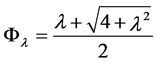 ,
,
![]() while for the first four positive integers
while for the first four positive integers
 we use the following names:
 is the golden proportion (the golden ratio),
 is the silver proportion,
 is the bronze proportion,
 is the cooper proportion.
The following functions are called the hyperbolic Fibonacci l-sinus
 and the hyperbolic Fibonacci l-cosine
 , respectively:
 (91)
(91)
Since![]() , we get the following relations between the classical hyperbolic
functions sh(x), ch(x) and Fibonacci l-functions
, we get the following relations between the classical hyperbolic
functions sh(x), ch(x) and Fibonacci l-functions ,
, :
:
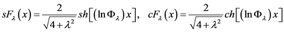 , (92)
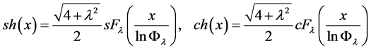 . (93)
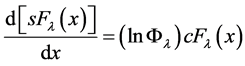
Such formulas are useful for differentiation and integration and derivation of other relations. Hence, for instance, we get:
 ,
,
 ,
,
 ,
,
 ,
,

In the terms of the “metallic proportions” and “hyperbolic Fibonacci functions,” the diffeomorphism (64) and the metric form (90) have the following forms:
 (94)
(94)
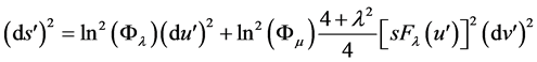 , (95)
where the old parameters
 is linked with the new parameters
 with the following relations:
 (96)
(96)
Recall that we assumed that the radius of the pseudo-sphere R = 1, and hence the
Gaussian curvature as the pseudo-sphere and all the metric forms discussed below
is equal to .
.
The two-parametric metric forms (95) are called Lobachevski’s metric (l, m)-forms.
In these terms, the distance
 between the Lobachevski’s metric (l, m)-forms (95) and Lobachevski’s classic metric
form (89) takes the following form:
between the Lobachevski’s metric (l, m)-forms (95) and Lobachevski’s classic metric
form (89) takes the following form:

Note that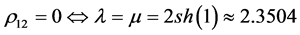 , that is, when
 , the (l, m)-metric forms (95) are
arbitrarily close to Lobachevski’s classic metric form (89).
, the (l, m)-metric forms (95) are
arbitrarily close to Lobachevski’s classic metric form (89).
In particular, if the parameters
 take only the integer values
 for the case
 , the metric forms (95) are called the
“pure Lobachevski’s metric (l, m)-forms,” and for the case
, the metric forms (95) are called the
“pure Lobachevski’s metric (l, m)-forms,” and for the case
 they are called the the “mixed Lobachevski’s metric (l, m)-forms.”
The pure Lobachevski’s metric ((, ()-forms:
1) The “golden” (l, m)-form for the case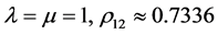 2) The “silver” (l, m)-form for the case
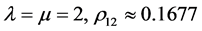 3) The “bronze” (l, m)-form for the case
 4) The “cooper” (l, m)-form for
the case
4) The “cooper” (l, m)-form for
the case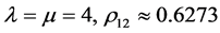 .
.
The mixed Lobachevski’s metric ((, ()-forms:
1) The “golden-silver” (l, m)-form for the case ,
,
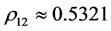
2) The “golden-bronze” (l, m)-form for the case ,
,
3) The “golden-cooper” (l, m)-form for the case ,
,
4) The “cooper-golden” (l, m)-form for the case ,
,

5) The “cooper-silver” (l, m)-form for the case ,
,
6) The “cooper-golden” (l, m)-form for the case ,
, .
.
12. Geodesic Lines of the Metric ((, ()-Forms of Lobachevski’s Plane and Other Geometric Objects
12.1. Preliminary Information
Let us consider the half-plane
 , where Lobachevski’s metric form (89) has the following form:
 .
.
To find the geodesic lines, we consider the surface:
 (97)
(97)
which is the upper half of the two-sheeted hyperboloid (pseudosphere of the radius
R = 1), embedded in the three-dimensional Euclidean space (X, Y, Z), having Minkowski’s
metric
 with the following parametrization of the surface (97) in the form:
![]() (98)
(98)
Geodesic lines L on
 can be found in the form of the intersection
 , where the П-surfaces pass through the
coordinate origin O(0, 0, 0) of the space (X, Y, Z)
, where the П-surfaces pass through the
coordinate origin O(0, 0, 0) of the space (X, Y, Z)
 (99)
(99)
Then the intersection
 satisfies to the system of equations:
 (100)
(100)
Let us consider two cases: 1) с = 0; 2)
![]()
For the case 1) с = 0, we get , that is, the geodesic lines are halflines
 (101)
(101)
For the case 2)
 we get:

Hence, we obtain the relations: , it follows from here that the geodesic
lines have the following arcs:
, it follows from here that the geodesic
lines have the following arcs:
 .
.
For other equivalent record, the last relation has the following form:
 , (102)
where
 .
.
The surface (97) , in addition to the parametrization
(98), also allows the parametrization of the following form:
, in addition to the parametrization
(98), also allows the parametrization of the following form:
![]() . (103)
. (103)
But then the diffeomorphism
 of half-surface
 of the kind


 converts the geodesic lines S
of the form (101) and (102) of Lobachevski’s metric form
converts the geodesic lines S
of the form (101) and (102) of Lobachevski’s metric form
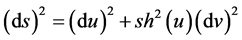 into the geodesic lines
 of the metric form
 .
.
In the coordinates
 the geodesic lines
 have the following form:
1) ,
,
 , if in (100) с = 0;
2) ,
,
 ,
,
 ,
,
![]()
In another equivalent record, the last relation can be rewritten as follows:
 (104)
(104)
where .
.
Therefore, the diffeomorphism
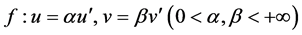 is geodesic mapping.
12.2. Presentation of the Geodesic Lines in the Terms of the “Metallic Proportions” and “Fibonacci Hyperbolic Geometry”
After replacing ,
,
 for the metric
 -form (104) the geodesic lines
 in the coordinates
 have the following form:
1) ,
,
 , if in (100) с = 0;
2)
 ,
,
 , if in (100)
![]() .
.
In other equivalent record the last relation can be rewritten as follows:
 (105)
(105)
where .
.
13. Poincare’s Model of Lobachevski’s Plane on the Unit Disc and Connection between Poincare’s Model of Lobachevski’s Plane and the ((, ()-Models of Lobachevski’s Plane
13.1. The Angles between the Curves for the Metrical Forms of General Form
For the completeness of presentation, we recall the well-known formulas of the internal geometry for each fixed metrical form
 ,
,
![]() Suppose that L1: u = u1 (t), v = v1
(t) and L2: u = u2 (t), v = v2 (t) are two smooth
arcs, which intersects at the value of the parameter t = 0 in the point (u0,
v0). Then, the angle
Suppose that L1: u = u1 (t), v = v1
(t) and L2: u = u2 (t), v = v2 (t) are two smooth
arcs, which intersects at the value of the parameter t = 0 in the point (u0,
v0). Then, the angle
![]() between these arcs in the point (u0, v0) is defined as follows:
between these arcs in the point (u0, v0) is defined as follows:
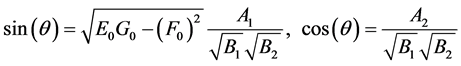 , (106)
where

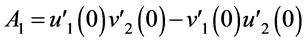 ,
,
 ,
,
 ,
,
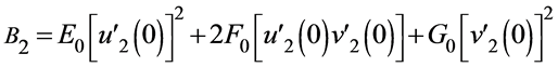
where
 is the operator of the derivative taking, dudv is the inner (scalar) product of
the differentials.
is the operator of the derivative taking, dudv is the inner (scalar) product of
the differentials.
The geodesic lines for Lobachevski’s metric form (89), as well as geodesic lines for Lobachevski’s metric
 -forms, which are on the distance
![]()
 from the metric form
(89), are a special case of such smooth curves on the half-plane ; while for Lobachevski’s metric form
(89), and for Lobachevski’s metric
; while for Lobachevski’s metric form
(89), and for Lobachevski’s metric
 -forms (95), the Gaussian curvature
 .
.
As indicated above, for the case
 the diffeomorphisms
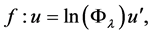
 , which convert the metric form (89) into the metric
forms (95), are not conformal, that is, not preserve angles due to the action of
the diffeomorphisms f between the relevant curves at the transition from Lobachevski’s
metric form (89) to Lobachevski’s metric
, which convert the metric form (89) into the metric
forms (95), are not conformal, that is, not preserve angles due to the action of
the diffeomorphisms f between the relevant curves at the transition from Lobachevski’s
metric form (89) to Lobachevski’s metric
 -forms (85).
The authors did not set out the goal to derive the relationships between all other
possible geometric and differential objects, induced by the metric
 -forms of the Gaussian curvative
 or the fixed Gaussian curvative
![]() on the half-plane
on the half-plane , which are on the distance
 from Lobachevski’s metric form at the changes of the parameters
 and which coincide with Lobachevski’s metric form for the case
 . This problem is the subject of a separate
study.
. This problem is the subject of a separate
study.
In connection with this problem, we consider only the model of Lobachevski’s plane
on the disk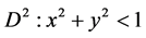 , proposed in 1882 by the great French
mathematician, physicist and astronomer Henri Poincare (1854-1912). We show its
relationship to Lobachevski’s metric
, proposed in 1882 by the great French
mathematician, physicist and astronomer Henri Poincare (1854-1912). We show its
relationship to Lobachevski’s metric
 -forms.
Let us remind the basic facts of Lobachevski’s geometry for Poincare’s realization
on the disc . The information is taken from [50].
Recall that for R = 1,
 , for this case the surface (60) has the form:

 and, according to [50]
, also it allows a parametrization of the kind:
and, according to [50]
, also it allows a parametrization of the kind:
 (107)
(107)
where![]() . For the variables (x, y) of Poincare’s metric form of
the Gaussian curvature
. For the variables (x, y) of Poincare’s metric form of
the Gaussian curvature
 is given by:
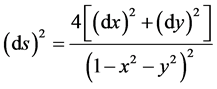 , (108)
where

 , dl is an arc element in the space (X, Y, Z) for the
surface
, dl is an arc element in the space (X, Y, Z) for the
surface ,
,
 is an arc element in the disc
 .
.
Since, according to (103), the surface (97)
 also admits a parametrization of the kind
![]() , where
, where

![]() , then
, then
 and
and
 are connected by relationships:
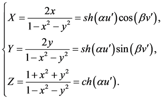 (109)
(109)
Hence, we obtain the following recalculation
![]() into
into![]() :
:
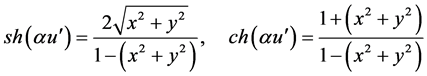 (110)
(110)
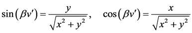 (111)
(111)
Inverse recalculation
![]() into
into
![]() gives the following result:
gives the following result:
 (112)
(112)
Then, we obtain the following correspondences:
 ,
,
 .
.
Recall that
 is the domain of Poincare’s metric form (108), for which the absolute is
 , and
, and
 is the domain of the definition of the two-parametric forms (90), for which the
absolute is the union:
is the domain of the definition of the two-parametric forms (90), for which the
absolute is the union:

It follows from this that the comparison by using the transformations (110)-(112)
of Poincare’s metric form (108), defined on the disc , with the two-parametric forms (90),
defined on the half-plane
, with the two-parametric forms (90),
defined on the half-plane
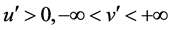
 , is possible only for the condition, when Poincare’s
metric form (108) is considered in the domain
, is possible only for the condition, when Poincare’s
metric form (108) is considered in the domain
 .
.
Then, under the action of the diffeomorphism (112), Poincare’s metric form (108),
which is considered, for this case, in the ring , is converted for each fixed values of
the parameters
, is converted for each fixed values of
the parameters
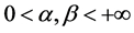 into the two-parametric form (90) by retaining the element of the arc length, that
is,
into the two-parametric form (90) by retaining the element of the arc length, that
is,
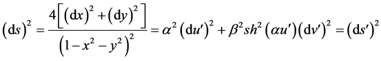 (113)
(113)
According to definition 1, the transformation (112) in this case is isometric mapping and the metric forms (108) and (90) are isometrically equivalent.
However, since for the variables (x, y) and
 the metric forms (108) and (90) are different, then the metric forms (108) and (90)
are not isometrically identical, and the transformation (112) is not an isometry
(see definition 2).
the metric forms (108) and (90) are different, then the metric forms (108) and (90)
are not isometrically identical, and the transformation (112) is not an isometry
(see definition 2).
Let
 and
and
 be arbitrary points of Lobachevski’s plane, which is realized in the form of a circle
 with the metrics (108).
Further we use complex numbers. We designate the point
 by
by , where
 is imaginary unit. A module of the complex number z is equal to
 . Let
. Let
 be a complex number conjugate to the complex number
 .
.
For this case the points
 and
and
 in complex notation can be represented as follows:
 . It is well-known that the distance
 between two points
 and
and
 in complex notation has the following form:
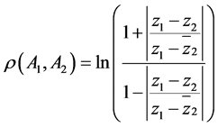 (114)
(114)
For the real variables , the formula (114) has the following
form [52] :
, the formula (114) has the following
form [52] :
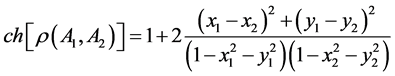 .
.
This implies that if in the area
 we fix the point
 , and
, and
![]() , that is
, that is
 “from within” the domain
 , then
 and therefore at approaching to the absolute, the distance
 , where
![]() is induced by Poincare’s metric form (108).
is induced by Poincare’s metric form (108).
In complex notation the metrics (108) has the following form:
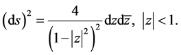 (115)
(115)
The movement of the metrics (108) of Lobachevski’s plane is written as follows:
 (116)
(116)
where
 and
and .
.
Note that at the movements (116) the metric form is saved, that is, if we consider the transformation
 , (117)
inverse with respect to the transformation (116), and then after the substitution of (117) into (115), we get the metric form
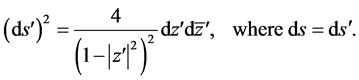 (118)
(118)
According to definition 2, the transformation (117) is an isometry and the metric form (115) and (118) are isometrically identical. Since any isometry is also a conformal transformation (see definitions 2 and 3), the transformation (116) preserves not only the elements of the arc lengths, but the angles between the arcs. Therefore, the metric forms (115) and (118) are also conformal metric forms, having the same conformal forms. The transformation (116) has similar properties.
Consider further the form of the geodesic lines in the coordinates
 for the metric form (108) and compare them with the geodesic lines in the coordinates
 for the metric form (90).
According to (100), the geodesic lines L on
 with
with
 satisfy to the conditions:

According to (107), the surface
 admits a parametrization:
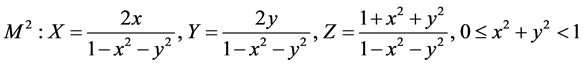 . (119)
Therefore, to find the geodesic lines S on the disc
 for the metric form (108), we should now consider the following system of equations:
 (120)
(120)
Then the equation of the geodesic lines
![]() for the metric form (108), after substitution
for the metric form (108), after substitution ,
,
 ,
,
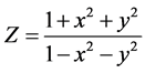 into the equation
 and reduceing the common factor
 , takes the following form:
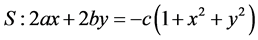 . (121)
Let us consider two cases: 1). с = 0; 2).
![]()
For the case 1) с = 0, the equation (121) for the geodesic lines S on the disc
 takes the following form:
 , that is, the geodesic lines S are the
line segments, belonging to the disc
, that is, the geodesic lines S are the
line segments, belonging to the disc .
.
For the case 2)
 the equation (121) takes the following form:
 , (122)
where ,
, .
.
Consequently, the geodesic lines on S for the case
![]() are arcs of the circles
are arcs of the circles
 , (123)
belonging to the disc
 . Note that the center
 of the circles (123) is outside of the disc
 . Direct verification establishes that
the circles (123) intersect with the absolute
. Direct verification establishes that
the circles (123) intersect with the absolute
 under the right angle.
13.2. The Relationship between Poincaré’s Metric Model and Lobachevski’s Metric ((, ()-Models
Assume that , then, we get:
 ,
,
 ,
,
 ,
,
 ,
,
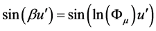 ,
, .
.
Hence, the formulas (110)-(113), obtained after recalculation in the terms of the
“metallic proportions” and “hyperbolic Fibonacci goniometry,” between Poincaré’s
metric model and Lobachevski’s metric
 -models, take the following forms:
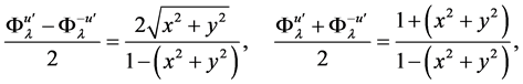 (124)
(124)
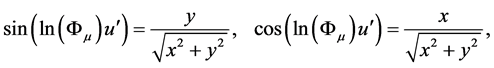 (125)
(125)
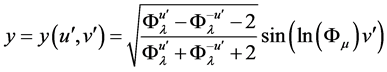 , (126)
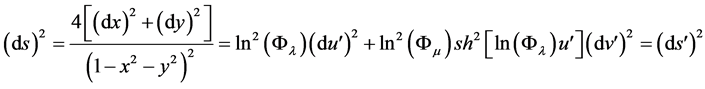 . (127)
14. The Main Results of the Study
14.1. The Original Solution of Hilbert’s Fourth Problem
Thus, Lobachevski’s metric
 -forms (95) give a countless set of geometries, based on the
“metallic proportions” and “hyperbolic Fibonacci goniometry”
[3]. On the one hand, they possess the properties, similar to Lobachevski’s
metric form (59), where
-forms (95) give a countless set of geometries, based on the
“metallic proportions” and “hyperbolic Fibonacci goniometry”
[3]. On the one hand, they possess the properties, similar to Lobachevski’s
metric form (59), where
 (preservation of the same Gaussian curvature
 , isometricaly equivalence, equiareality on the other
hand, when compared with Lobachevski’s metric form (59), where
, isometricaly equivalence, equiareality on the other
hand, when compared with Lobachevski’s metric form (59), where , they have their specific properties (non-conformal,
if
, they have their specific properties (non-conformal,
if , and non-isometrical)
If at least one of the values
![]() or
or
![]() not equal to
not equal to , Lobachevski’s metric
 -forms (95) are on the finite distance
 from Lobachevski’s metric
 -forms (95), moreover, for the case
 , the distance
 .
.
This means that for the case
 Lobachevski’s metric
 -forms (95) are arbitrarily close to Lobachevski’s metric
form (59) and coincide with (59) for the case
-forms (95) are arbitrarily close to Lobachevski’s metric
form (59) and coincide with (59) for the case .
.
It is clear that these new Lobachevski’s geometries “with equal right, stand next to Euclidean geometry” (David Hilbert). It follows from this consideration that the formula (95) can be considered as the partial original solution to Hilbert’s Fourth Problem. That is, there are an infinite number of Lobachevski’s geometries, described by the formula (95), which are close to Euclidean geometry.
Each of these new Lobachevski’s geometries, based on the “metallic proportions” and “hyperbolic Fibonacci goniometry,” can actually exist in the real physical world, similarly to “Bodnar’s geometry” [8] , which is a unique hyperbolic geometry of botanical phenomenon of phyllotaxis, widely common in wildlife. As it is proved in [8] , the hyperbolic geometry of phyllotaxis is based on the classical “golden ratio” and Fibonacci numbers, which appear at the surface of phyllotaxis objects.
14.2. A New Challenge for Theoretical Natural Sciences
Thus, the main result of the research, described in [18] [19] , is a proof
of the existence of an infinite number of hyperbolic functions, Fibonacci hyperbolic
l-functions, based on the “metallic proportions” (35). For the given
 each class of the Fibonacci hyperbolic l-functions, “generates” new hyperbolic geometry,
which leads to the appearance in the “physical world” specific hyperbolic geometries
with properties, which depend on the “metallic proportions” (35). The new geometric
theory of phyllotaxis, created by Oleg Bodnar
[8] , is a striking example
of this. Bodnar proved that “the world of phyllotaxis” is a specific “hyperbolic
world,” in which a “hyperbolicity” manifests itself in the “Fibonacci spirals” on
the surface of “phyllotaxis objects”.
each class of the Fibonacci hyperbolic l-functions, “generates” new hyperbolic geometry,
which leads to the appearance in the “physical world” specific hyperbolic geometries
with properties, which depend on the “metallic proportions” (35). The new geometric
theory of phyllotaxis, created by Oleg Bodnar
[8] , is a striking example
of this. Bodnar proved that “the world of phyllotaxis” is a specific “hyperbolic
world,” in which a “hyperbolicity” manifests itself in the “Fibonacci spirals” on
the surface of “phyllotaxis objects”.
Recall that “Bodnar’s geometry” [8] is based on the Fibonacci hyperbolic functions, also known as the “golden” hyperbolic functions:
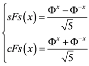 (128)
(128)
which are connected with Fibonacci numbers according to the relation (18).
The famous irrational number
 is the base of the functions (128). The distance of “Bodnar’ geometry” to Lobachevski’s
geometry is equal
is the base of the functions (128). The distance of “Bodnar’ geometry” to Lobachevski’s
geometry is equal .
.
However, the “golden” hyperbolic functions (128), which underlie the “hyperbolic
phyllotaxis world,” are a special case of the hyperbolic Fibonacci l-functions . In this regard, there is every reason to suppose that
other types of hyperbolic functions, Fibonacci hyperbolic l-functions, can be the
basis for modeling of new “hyperbolic worlds” that can really exist in Nature. Modern
science could not find these special “hyperbolic worlds,” because the Fibonacci
hyperbolic l-functions were unknown until the 21st century. For the first time,
these hyperbolic functions are described in Stakhov’s 2006 article [18] and then in Stakhov’s and Aranson’s
2011 articles [20] [21]
. Basing on the success of “Bodnar’s geometry”
[8] , one can put forward in
front to theoretical physics, chemistry, crystallography, botany, biology, and other
branches of theoretical natural sciences the challenge to find new (“harmonic”)
hyperbolic worlds of Nature, based on other classes of the Fibonacci hyperbolic
l-functions (16), (17).
. In this regard, there is every reason to suppose that
other types of hyperbolic functions, Fibonacci hyperbolic l-functions, can be the
basis for modeling of new “hyperbolic worlds” that can really exist in Nature. Modern
science could not find these special “hyperbolic worlds,” because the Fibonacci
hyperbolic l-functions were unknown until the 21st century. For the first time,
these hyperbolic functions are described in Stakhov’s 2006 article [18] and then in Stakhov’s and Aranson’s
2011 articles [20] [21]
. Basing on the success of “Bodnar’s geometry”
[8] , one can put forward in
front to theoretical physics, chemistry, crystallography, botany, biology, and other
branches of theoretical natural sciences the challenge to find new (“harmonic”)
hyperbolic worlds of Nature, based on other classes of the Fibonacci hyperbolic
l-functions (16), (17).
In this case, perhaps, the first candidate for the new “hyperbolic world” of Nature may be, for example, “silver” hyperbolic functions:
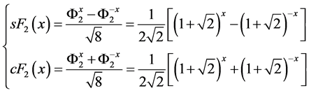 , (129)
which are connected with Pell numbers [34] and
are based on the “silver mean” , connected with the fundamental mathematical
constant
, connected with the fundamental mathematical
constant .
.
In this regard, we should pay a special attention to the fact that the new hyperbolic
geometry, based on the “silver” hyperbolic functions (129), is the closest to Lobachevski’s
geometry, based on the classical hyperbolic functions (15) with the base![]() . Its distance to Lobachevski’s geometry
is equal
. Its distance to Lobachevski’s geometry
is equal
 what is the lowest among all the distances for Lobachevski’s metric
 -forms, where in this case the parameters
 take the values
 .
.
It may assume that the “silver” hyperbolic functions (129) and the generating by them “silver” hyperbolic geometry can be soon be found in nature and the “silver” hyperbolic geometry can take its rightful place in modern science next to “Bodnar’s geometry,” based on the “golden” hyperbolic functions (128).
15. General Conclusions
1) Discussing the history of mathematics and the development of new mathematical ideas and theories, we should pay a particular attention to the great role of Euclid’s Elements in this process. Academician Andrei Kolmogorov identifies several stages in the development of mathematics [2] . According to Kolmogorov, the beginning of modern mathematics refers to the 19th century. Expanding the object of mathematics became the most significant feature of the 19th century mathematics. At the same time, according to Kolmogorov, the creation of Lobachevski’s “imaginary geometry” became “a remarkable example of the theory that has arisen as a result of internal development of mathematics... It is an example of the geometry, which overcame a belief in the permanence of the axioms, consecrated millennial development of mathematics, and gave a comprehension of the possibility of creating significant new mathematical theories... [2] . As we know, the “hyperbolic geometry” in its origins dates back to Euclid’s 5th postulate. For several centuries, from Ptolemy and Proclus, mathematicians tried to prove this postulate. First, a brilliant solution to the problem was given by Russian mathematician Nikolai Lobachevski in the first half of the 19th century. This became the beginning of contemporary stage in the development of mathematics.
2) At the turn of the 19th and 20th century, the eminent mathematician David Hilbert formulated 23 mathematical problems, which largely stimulated the development of mathematics in the 20 century. One of them (Hilbert’s Fourth Problem) refers directly to the hyperbolic geometry. Gilbert put forth for mathematicians the following fundamental problem [42] : “The more general question now arises: whether from other suggestive standpoints geometries may not be devised which, with equal right, stand next to Euclidean geometry.” Hilbert’s quote contains the formulation of a very important scientific problem, which has fundamental importance not only for mathematics, but also for all theoretical natural sciences: are there non-Euclidean geometries, which are close to the Euclidean geometry and are interesting from the “other suggestive standpoints?” If we consider it in the context of theoretical natural sciences, then Hilbert’s Fourth Problem is about finding NEW HYPERBOLIC WORLDS OF NATURE, which are close to the Euclidean geometry and reflect some new properties of Nature’s structures and phenomena. Unfortunately, the efforts of mathematicians to solve this problem have not led to substantial progress. In modern mathematics there is no consensus on the solution to this problem. In mathematical literature Hilbert’s Fourth Problem is sometimes considered as formulated very vague what makes difficult its final solution. As it is noted in Wikipedia [44] , “the original statement of Hilbert, however, has also been judged too vague to admit a definitive answer.”
3) Besides 5th postulate, Euclid’s Elements contain another fundamental idea that permeates the entire history of science. We are talking about the “idea of the Universe Harmony,” which in ancient Greece was associated with the “golden ratio” and Platonic solids. “Proclus hypothesis,” formulated in the 5th century AD by the famous Greek philosopher and mathematician Proclus Diadochus (412-485), contains the unexpected view on Euclid’s “Elements”. According to Proclus, Euclid’s main goal was to build a full theory of regular polyhedra (“Platonic solids”). This theory was set forth by Euclid in the XIII-th, that is, in the final book of the “Elements” what in itself is an indirect confirmation of “Proclus’ hypothesis.” To solve this problem, Euclid had included the necessary mathematical information into his Elements. The most curious thing is that he had introduced in Book II the “golden ratio” for the creation of geometric theory of the dodecahedron.
4) Starting with Euclid, the “golden ratio” and “Platonic solids” permeate by the “red thread” through the history of mathematics and theoretical natural sciences. In modern science, Platonic solids have become a source for new scientific discoveries, particularly fullerenes (Nobel Prize in Chemistry, 1996) and quasi-crystals (Nobel Prize in Chemistry, 2011). Publication of Stakhov’s book “The Mathematics of Harmony, from Euclid to Contemporary Mathematics and Computer Science” [3] is a reflection of the very important trend in the development of modern science (including mathematics)—the revival of “harmonic ideas” of Pythagoras, Plato and Euclid.
5) The “metallic proportions” by Vera de Spinadel [26] , which are a generalization of the classical “golden ratio,” are new classes of mathematical constants, representing fundamental theoretical and practical interest. Besides Argentinean mathematician Vera de Spinadel, many researchers from different countries and continents (French mathematician Midhat Gazale [27] , American mathematician Jay Kappraff [28] , Russian engineer Alexander Tatarenko [29] , Armenian philosopher and physicist Hrant Arakelyan [30] , Russian researcher Victor Shenyagin [31] , Ukrainian physicist Nikolai Kosinov [32] , Spanish mathematicians Falcon Sergio and Plaza Angel [33] and others) independently came to this mathematical result.
6) New classes of hyperbolic functions, based on the “golden ratio” and Fibonacci
numbers (hyperbolic Fibonacci and Lucas functions), became one of the most important
results of the “mathematics of harmony” of direct relevance to the hyperbolic geometry.
First this mathematical result has been obtained by the Ukrainian mathematicians
Alexey Stakhov, Ivan Tkachenko, Boris Rosin [14]
-[17] . Further development of the theory of hyperbolic
functions becomes hyperbolic lambda Fibonacci and Lucas functions, based on the
“metallic proportions.” Hyperbolic Fibonacci and Lucas
![]() -functions, based on the “metallic proportions” and introduced
by Alexey Stakhov in 2006 [18]
, are a further development of the general theory of hyperbolic functions
[19] .
-functions, based on the “metallic proportions” and introduced
by Alexey Stakhov in 2006 [18]
, are a further development of the general theory of hyperbolic functions
[19] .
7) Researches of the Ukrainian architect Oleg Bodnar are a significant result in the development of the “hyperbolic geometry”. Bodnar showed [8] that a special type of hyperbolic geometry, based on the “golden” hyperbolic functions (128), is distributed widely in Nature and is the basis of the “phyllotaxis geometry” (pine cones, cacti, pineapples, sunflower heads, etc.).
8) The original solution of Hilbert’s Fourth Problem, based on the “mathematics
of harmony” by Alexey Stakhov [3]
, in particular, on Spinadel’s “metallic proportions” and hyperbolic Fibonacci
![]() -functions [18]
[19] , is the main result of
this article and the previous works of the authors [20] -[23] . It
is proved in these works that there are an infinite number of new hyperbolic geometries
that “with equal right, stand next to Euclidean geometry” (David Hilbert). This
is the original solution of Hilbert’s Fourth Problem, developed in this article
and the articles [20] -[23] . This approach poses in front to theoretical natural
sciences (physics, chemistry, biology, genetics and so on) the theoretical problem
of finding new (“harmonic”) worlds of Nature, which can objectively exist in the
world around us. In this regard, we should pay a special attention to the fact that
the new hyperbolic geometry, based on the “silver” hyperbolic functions (129) with
the base
-functions [18]
[19] , is the main result of
this article and the previous works of the authors [20] -[23] . It
is proved in these works that there are an infinite number of new hyperbolic geometries
that “with equal right, stand next to Euclidean geometry” (David Hilbert). This
is the original solution of Hilbert’s Fourth Problem, developed in this article
and the articles [20] -[23] . This approach poses in front to theoretical natural
sciences (physics, chemistry, biology, genetics and so on) the theoretical problem
of finding new (“harmonic”) worlds of Nature, which can objectively exist in the
world around us. In this regard, we should pay a special attention to the fact that
the new hyperbolic geometry, based on the “silver” hyperbolic functions (129) with
the base , is the closest to Lobachevski’s geometry,
based on the classical hyperbolic functions (15) with the base
, is the closest to Lobachevski’s geometry,
based on the classical hyperbolic functions (15) with the base![]() . Its distance to Lobachevski’s geometry
is equal
. Its distance to Lobachevski’s geometry
is equal
 what is the lowest among all the distances for Lobachevski’s metric
 -forms. We may assume that the “silver” hyperbolic functions
(129) and the generating by them “silver” hyperbolic geometry can take its rightful
place in modern science next to “Bodnar’s geometry,” based on the “golden” hyperbolic
functions (128).
-forms. We may assume that the “silver” hyperbolic functions
(129) and the generating by them “silver” hyperbolic geometry can take its rightful
place in modern science next to “Bodnar’s geometry,” based on the “golden” hyperbolic
functions (128).
9) A study in this article is of considerable interest from the standpoint of the mathematics history and prospects of its development in close association with the theoretical natural sciences. This study unites the ancient “golden ratio,” described in Euclid’s Elements, with Lobachevski’s hyperbolic geometry, rising back in its origins to Euclid’s 5th postulate. This union led to the original solution of Hilbert’s Fourth Problem what is the very important mathematical result, which opens the new (“harmonic”) stage in the development of hyperbolic geometry and its applications in theoretical natural sciences.
References
- Wikipedia, the Free Encyclopaedia (2014) Hyperbolic Geometry. http://en.wikipedia.org/wiki/Hyperbolic_geometry
- Kolmogorov, A.N. (1991) Mathematics in Its Historical Development (in Russian). Nauka, Moscow.
- Stakhov, A.P. (2009) The Mathematics of Harmony. From Euclid to Contemporary Mathematics and Computer Science. International Publisher “World Scientific”, New Jersey, London, Singapore, Beijing, Shanghai, Hong Kong, Taipei, Chennai.
- Stakhov, A.P. (2008) The Mathematics of Harmony: Clarifying the Origins and Development of Mathematics. Congressus Numerantium, CXCIII, 5-48.
- Wikipedia, the Free Encyclopaedia (2014) Fullerene. http://en.wikipedia.org/wiki/Fullerene
- Wikipedia, the Free Encyclopaedia (2014) Quasi-Crystal. http://en.wikipedia.org/wiki/Quasicrystal
- Soroko, E.M. (1984) Structural Harmony of Systems (in Russian). Publishing House “Nauka i Tekhnika,” Minsk.
- Bodnar, O.Y. (1994) The Golden Section and Non-Euclidean Geometry in Nature and Art (in Russian). Publishing House “Svit”, Lvov.
- Bodnar, O. (2010) Dynamic Symmetry in Nature and Architecture. Visual Mathematics, 12, 4. http://www.mi.sanu.ac.rs/vismath/BOD2010/index.html
- Bodnar, O. (2011) Geometric Interpretation and Generalization of the Non-Classical Hyperbolic Functions. Visual Mathematics, 13, 2. http://www.mi.sanu.ac.rs/vismath/bodnarsept2011/SilverF.pdf
- Bodnar, O. (2012) Minkovski’s Geometry in the Mathematical Modeling of Natural Phenomena. Visual Mathematics, 14, 1. http://www.mi.sanu.ac.rs/vismath/bodnardecembar2011/mink.pdf
- Wikipedia, the Free Encyclopedia (2014) Hilbert’s Tenth Problem. http://en.wikipedia.org/wiki/Hilbert’s_tenth_problem
- Petoukhov, S.V. (2006) Metaphysical Aspects of the Matrix Analysis of Genetic Code and the Golden Section. Metaphysics: Century XXI (in Russian). Publishing House “BINOM”, Moscow, 216-250.
- Stakhov, A.P. and Tkachenko, I.S. (1993) Hyperbolic Fibonacci Trigonometry (in Russian). Reports of the Ukrainian Academy of Sciences, 208, 9-14.
- Stakhov, A. and Rozin, B. (2004) On a New Class of Hyperbolic Function. Chaos, Solitons & Fractals, 23, 379-389.
- Stakhov, A. and Rozin, B. (2007) The “Golden” Hyperbolic Models of Universe. Chaos, Solitons & Fractals, 34, 159-171.
- Stakhov, A.P. and Rozin, B.N. (2006) The Golden Section, Fibonacci Series and New Hyperbolic Models of Nature. Visual Mathematics, 8, 3. http://www.mi.sanu.ac.rs/vismath/stakhov/index.html
- Stakhov, A.P. (2006) Gazale formulas, a New Class of the Hyperbolic Fibonacci and Lucas Functions, and the Improved Method of the “Golden” Cryptography. Academy of Trinitarizam, Moscow. http://www.trinitas.ru/rus/doc/0232/004a/02321063.htm
- Stakhov, A. (2013) On the General Theory of Hyperbolic Functions Based on the Hyperbolic Fibonacci and Lucas Functions and on Hilbert’s Fourth Problem. Visual Mathematics, 15, 1. http://www.mi.sanu.ac.rs/vismath/pap.htm)
- Stakhov, A. and Aranson, S. (2011) Hyperbolic Fibonacci and Lucas Functions, “Golden” Fibonacci Goniometry, Bodnar’s Geometry, and Hilbert’s Fourth Problem. Part I. Applied Mathematics, 2, 74-84. http://dx.doi.org/10.4236/am.2011.21009
- Stakhov, A. and Aranson, S. (2011) Hyperbolic Fibonacci and Lucas Functions, “Golden” Fibonacci Goniometry, Bodnar’s Geometry, and Hilbert’s Fourth Problem. Part II. Applied Mathematics, 2, 181-188. http://dx.doi.org/10.4236/am.2011.22020
- Stakhov, A. and Aranson, S. (2011) Hyperbolic Fibonacci and Lucas Functions, “Golden” Fibonacci Goniometry, Bodnar’s Geometry, and Hilbert’s Fourth Problem. Part III. Applied Mathematics, 2, 283-293. http://dx.doi.org/10.4236/am.2011.23033
- Stakhov, A.P. (2013) Hilbert’s Fourth Problem: Searching for Harmonic Hyperbolic Worlds of Nature. Applied Mathematics and Physics, 1, 60-66. http://www.scirp.org/journal/jamp/.
- Stakhov, A.P. (1984) Codes of the Golden Proportion (in Russian). Publishing House “Radio and Communications”, Moscow, 1984.
- Shervatov, V.G. (1958) Hyperbolic Functions (in Russian). Fizmatgiz, Moscow.
- de Spinadel, V.W. (2004) From the Golden Mean to Chaos. 2nd Edition, Nueva Libreria, Nobuko.
- Gazale, M.J. (1999) Gnomon. From Pharaohs to Fractals. Princeton University Press, Princeton.
- Kappraff, J. (2001) Connections. The Geometric Bridge between Art and Science. 2nd Edition, World Scientific, Singapore, New Jersey, London, Hong Kong.
- Tatarenko, A. (2005) The Golden -Harmonies’ and -fractals (in Russian). Academy of Trinitarism, Moscow. http://www.trinitas.ru/rus/doc/0232/009a/02320010.htm
- Arakelyan, H. (1989) The Numbers and Magnitudes in Modern Physics (in Russian). Publishing House “Armenian Academy of Sciences”, Yerevan.
- Shenyagin, V.P. (2011) Pythagoras, or How Everyone Creates His Own Myth. The Fourteen Years after the First Publication of the Quadratic Mantissa’s Proportions (in Russian). Academy of Trinitarism, Moscow. http://www.trinitas.ru/rus/doc/0232/013a/02322050.htm
- Kosinov, N.V. (2007) The Golden Ratio, Golden Constants, and Golden Theorems (in Russian). Academy of Trinitarism, Moscow. http://www.trinitas.ru/rus/doc/0232/009a/02321049.htm
- Falcon, S. and Plaza, A. (2007) On the Fibonacci k-numbers. Chaos, Solitons & Fractals, 32, 1615-1624. http://dx.doi.org/10.1016/j.chaos.2006.09.022
- Wikipedia, the Free Encyclopedia (2014) Pell Number. http://en.wikipedia.org/wiki/Pell_number
- Stakhov, A.P. (2012) A Generalization of the Cassini Formula. Visual Mathematics, 14, 2. http://www.mi.sanu.ac.rs/vismath/stakhovsept2012/cassini.pdf
- Aranson, S.Kh. (2000) Qualitative Properties of Foliations on Closed Surfaces. Journal of Dynamical and Control Systems, 6, 127-157. http://dx.doi.org/10.1023/A:1009525823422
- Aranson, S.Kh. and Zhuzoma, E.V. (2004) Nonlocal Properties of Analytic Flows on Closed Orientable Surfaces. Proceedings of the Steklov Institute of Mathematics, 244, 2-17.
- Aranson, S., Medvedev, V. and Zhuzhoma, E. (2000) Collapse and Continuity of Geodesic Frameworks of Surface Foliations. In: Andronov-Leontovich, E.A., Ed., Methods of Qualitative Theory of Differential Equations and Related Topics, American Mathematical Society, 200, 35-49.
- Aranson, S.Kh., Belitsky, E.V. and Zhuzhoma (1996) Introduction to the Qualitative Theory of Dynamical Systems on surfaces. American Mathematical Society.
- Anosov, D.V., Aranson, S.Kh., Arnold, V.I., Bronshtein, I.U., Grines, V.Z. and Il’yashenko, Yu.S. (1997) Ordinary Differential Equations and Smooth Dynamical Systems. Springer, Berlin.
- Anosov, D.V., Aranson, S.Kh., Grines, V.Z., Plykin, R.V., Safonov, A.V., Sataev, E.A., Shlyachkov, S.V., Solodov, V.V., Starkov, A.N. and Stepin, A.M. (1995) Dynamical Systems with Hyperbolic Behaviour. Encyclopaedia of Mathematical Sciences. Dynamical Systems IX, 66, Springer, Berlin, 1-235. http://dx.doi.org/10.1007/978-3-662-03172-8
- Hilbert, D. (1976) Mathematical Developments Arising from Hilbert’s Problems, American Mathematical Society. http://aleph0.clarku.edu/~djoyce/hilbert/problems.html#prob4
- Alexandrov’s, P.S. (1969) Hilbert’s Problems. Nauka, Moscow.
- Wikipedia, the Free Encyclopaedia (2003) Hilbert’s Fourth Problem.
- Busemann, H. (1966) On Hilbert’s Fourth Problem. Russian Mathematical Surveys, 21.
- Busemann, H. (1966) On Hilbert’s Fourth Problem (in Russian). Uspechi mathematicheskich nauk, 21, 155-164.
- Pogorelov, A.V. (1974) Hilbert’s Fourth Problem (in Russian). Nauka, Moscow.
- Aranson, S.Kh. (2009) Once again on Hilbert’s Fourth Problem (in Russian). Academy of Trinitarizm, Мoscow. http://www.trinitas.ru/rus/doc/0232/009a/02321180.htm
- Yandell, B.H. (2003) The Honors Class-Hilbert’s Problems and Their Solvers.
- Stakhov, A.P. (2013) Non-Euclidean Geometries. From the “Game of Postulates” to the “Game of Function (in Russian).” Academy of Trinitarizm, Мoscow. http://www.trinitas.ru/rus/doc/0016/001d/00162125.htm
- Dubrovin, B.A., Novikov, S.P. and Fomenko, A.T. (1979) Modern Geometry. Methods and Applications (in Russian). Nauka, Moscow.
- Arnold, V.I., II’yashenko, Yu.S., Anosov, D.V., Bronshtein, I.U., Aranson, S.Kh. and Grines, V.Z. (1998) Dynamical Systems I, Encyclopaedia of Mathematical Sciences. Springer-Verlag, Berlin.
- Kovantsov, N.I., et al. (1982) Differential Geometry, Topology, Tensor Analysis (in Russian). Higher School, Kiev.