International Journal of Intelligence Science
Vol.3 No.3(2013), Article ID:33968,10 pages DOI:10.4236/ijis.2013.33014
Forecast Urban Air Pollution in Mexico City by Using Support Vector Machines: A Kernel Performance Approach
Universidad Autónoma de Querétaro, Cerro de las Campanas S/N, Querétaro, México
Email: marco.aceves@gmail.com, artemiosotomayor@gmail.com
Copyright © 2013 Artemio Sotomayor-Olmedo et al. This is an open access article distributed under the Creative Commons Attribution License, which permits unrestricted use, distribution, and reproduction in any medium, provided the original work is properly cited.
Received January 26, 2013; revised March 18, 2013; accepted April 25, 2013
Keywords: Predictive Models; Airborne Pollution; Support Vector Machines; Kernel Functions
ABSTRACT
The development of forecasting models for pollution particles shows a nonlinear dynamic behavior; hence, implementation is a non-trivial process. In the literature, there have been multiple models of particulate pollutants, which use softcomputing techniques and machine learning such as: multilayer perceptrons, neural networks, support vector machines, kernel algorithms, and so on. This paper presents a prediction pollution model using support vector machines and kernel functions, which are: Gaussian, Polynomial and Spline. Finally, the prediction results of ozone (O3), particulate matter (PM10) and nitrogen dioxide (NO2) at Mexico City are presented as a case study using these techniques.
1. Introduction
In recent times, urban air pollution has been a growing problem especially for urban communities. Size, shape and chemical properties govern the lifetime of particles in the atmosphere and the site of deposition within the respiratory tract. Health effects differ upon the size of airborne particulates [1]. In this contribution, PM10 (particles less or equal than 10 micrometers) and PM2.5 (particles less or equal than 2.5 micrometers), Ozone and Nitrogen dioxide are considered due to its effect on human health. This is the primary reason why this research has been done: to monitor, and model the levels and spread of harmful particles in urban environments.
In previous contributions, it has been shown that forecast of concentration levels of PM10 may be possible by using other techniques such as neural networks and various fuzzy clustering algorithms [2]. However, there are other harmful particles such as Ozone and Nitrogen dioxide, making it essential to accurately model the nonlinear behavior of the system, by designing a more robust model with an enhanced method to reduce the error between the raw data and the model. For this reason, support vector machines (SVM) are chosen for this work. In this appraisal, the non-lineal behavior will be modeled using support vector machines working in regression mode.
Support vector machines are a recent statistical learning technique, based on machine learning and generalizetion theories, it implies an idea and could be considered as a method to minimize the risk.
A kernel approach is discussed, and the results for the forecast at Mexico City are illustrated. This is carried out using PM10 particles O3 and SO2. Finally, the results obtained by SVM kernel algorithms are validated using the raw data from the monitoring stations located at various sites in Mexico City.
Mexico City is one of the largest urban areas in the world, with over 20 million inhabitants within the city and an annual growth rate of between 3.3% and 5%. Also, Mexico City has an area of approximately 1300 km2 and is naturally open to the north and enclosed by mountains, 1000 m in height above the city, to the south, east and west. As most large cities located in valleys and surrounded by mountains, it has air pollution problems for certain particles.
Mexico City is a dry region of moderate climate with a diurnal pattern of winds blowing from the northwest and the northeast. The rainy season lasts from June to October. The industrial area comprises more than 30% of the whole national industry and is mostly located in the northern sectors of the city.
The high levels of fine particulate matter in Mexico City are of concern since they may induce severe public health effects [1].
2. Related Work
In this section, a list of significant works on soft computing, machine learning and computational methods designed for urban airborne pollution forecasting are listed. Several of this works present a mixture of methods such as neural networks, support vector machines and fuzzy inference systems, with other techniques.
For instance, Kolehmainen [3] has constructed a model using Self-Organized Map (SOM), Sammon’s mapping and fuzzy distance metrics to forecast levels of NO2, CO and PMx, while works such as the one carried out by Pokrovsky [4] shows a fuzzy logic based method to study the impact of meteorological factors on the evolution of air pollutant levels in order to describe them quantitatively.
Furthermore, some authors have focused their efforts on forecasting levels of airborne pollutants using various methods of artificial neural networks (ANN) [5-8].
In general, soft computing models were carried out using a mixture of two models such as: Box-Jenkins methods and ANN [9], Hidden Markov Model with Fuzzy Logic [10].
In previous contributions, urban air pollution models have been carried out using different fuzzy clustering techniques and fuzzy inference systems on particulate matter of less than 10 µm in diameter (PM10) [2].
Lastly, in terms of forecasting airborne pollution using support vector machines the work of Osowski [11] can be mentioned. In this work, the authors present a method for daily air pollution forecasting by using SVMs and wavelet decomposition. However, in such work only Gaussian kernel is shown.
In this contribution, support vector machines are used to construct models to forecast pollution levels using dissimilar particles, to determine performance for the kernels used (Gaussian, Polynomial and Spline).
3. Background
3.1. Urban Airborne Pollution
The health impact of air pollution became apparent during episodes in the USA and Europe in 1952 and 1958. Subsequent analysis of date for the London winters of 1958-1971 demonstrated that mortality and morbidity were associated with air pollution. The ability to measure the environmental health effects of pollution has improved over the last several decades, owing to advances in pollution monitoring and in statistical techniques [12].
The sources of air pollutants are numerous and varied. Three categories of sources may be defined: 1) natural (those that are not associated with human activities); 2) anthropogenic (those produced by human activities); and 3) secondary (those formed in the atmosphere from natural and anthropogenic air pollutants) [13].
Most major pollutants can alter pulmonary function in addition to other health effects when the exposure concentrations are high. This is especially severe in vulnerable sectors of the population such as children asthmatic and the elderly and has been vastly documented [14-17].
In this work, five particles were chosen due to the site’s availability and toxicity: Ozone, Nitrogen Dioxide (NO2) and Particulate Matter of less than 10 micrometers in diameter (PM10). The datasets are separated according to month of the year and type of particle. There is one data for each hour, for each particle for all five sites, making it difficult to extract information from datasets using commonly used methods, hence the importance to use novel methods for data extraction and analysis such as the one used in this work, especially when dealing with the non-linear behavior of airborne particle concentration.
3.1.1. Ozone
Ozone is a natural atmosphere component that is found on low concentrations and is crucial for life. Air pollution caused by high concentration of ozone is a common problem in large cities throughout the world [18].
Mexico City is among the ones suffering from this problem. It is a well-known fact that individuals exposed for a long period of time to high concentration of ozone may experience serious health problems [19]. Epidemiology studies have found associations between daily ozone levels and the hospital admission [20]. This pollutant is associated with respiratory symptoms specially coughing. This is aggravated in patients with asthma [21].
3.1.2. Nitrogen Dioxide
Nitrogen Dioxide (NO2) is a particularly important compound, not only for its health effects, but also because absorbs visible light and contributes to the visibility decrease. It also plays a critical role in production of ozone because the photolysis of NO2 is the initial step in the photochemical reaction of the ozone [13,18].
In nature, there is a nitrogen dioxide concentration of 10 to 50 parts per billion (ppb). However, the high levels of nitrogen dioxide are due to industrial processes and fossil sources. Furthermore, motor vehicles substantially contribute to urban levels of nitrogen oxides through their engine combustion processes [22]. According to several authors, the monitoring of NO2 is critically important, in order to assess the potential effect of NO2 on human health and ecosystems, as well as developing strategies for the effective control of NO2 pollution [23- 25].
3.1.3. PM10
The airborne particulate matter (PM) is a mixture of small particles and liquid droplets suspended in the atmosphere, which contributes significantly to the urban air quality such as acid rain and visibility degradation [26].
In airborne pollution, these particles could be any solid or liquid materials with a diameter between 0.002 and 500 micrometers (µm). Airborne particulates of 10 μm diameter and less are of concern from the perspective of air pollution [27]. A variety of national and worldwide standards, directives and guidelines exist to define acceptable particulate levels in the air. These types of particles are classified according to their effect on human health and their physical characteristics [28,29].
3.2. Support Vector Machines
The support vector machines (SVM) theory was developed by Vapnik [30]. This method is applied in many machine-learning applications such as object classification, time series prediction, regression analysis and pattern recognition. Support vector machines (SVM) are based on the principle of structured risk minimization (SRM) [31,32].
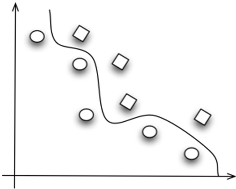
In the analysis using SVM, the main idea is to map the original data x into a feature space F with higher dimensionality via non-linear mapping function f, as shown in Figure 1, which is generally unknown, and then carry on linear regression in the feature space [33,34].
Thus, the regression approximation addresses a problem of estimating function based on a given data set (where xi represent the input vectors, di are the desired values), which is produced from the f function. SVM method approximates the function by:
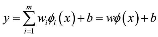 (1)
(1)
where w = [w1,···,wm] represent the weights vector, b are the bias coefficients and f(x) = [f1(x),···,fm(x)] the basis function vector.
The learning task is transformed to the weights of the network at minimum. The error function is defined through the e-insensitive loss function, Le(d,y(x)) and is given by:
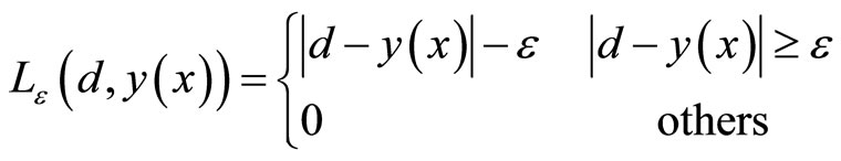 (2)
(2)
 (a)
(a)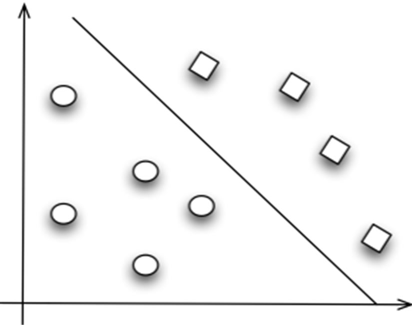 (b)
(b)
Figure 1. Feature map can simplify the classification and regression tasks. (a) Input space; (b) Feature space.
The solution of the so defined optimization problem is solved by the introduction of the Lagrange multipliers  (where
 ) responsible for the functional constraints defined in Equation (2). The minimizetion of the Lagrange function has been changed to the dual problem [35]
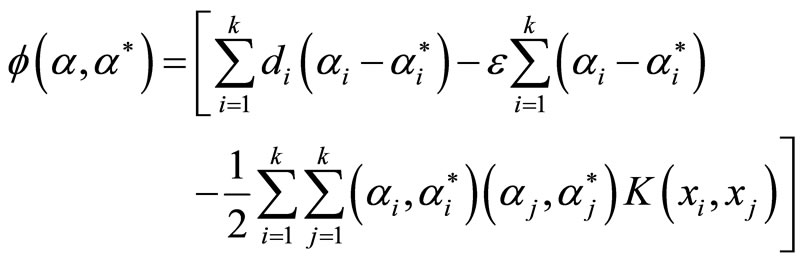 (3)
(3)
With constraints:
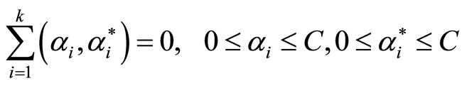 (4)
(4)
where C is a regularized constant that determines the trade-off between the training risk and the model uniformity.
According to the nature of quadratic programming, only those data corresponding to non-zero  pairs can be referred to support vectors. In Equation 3
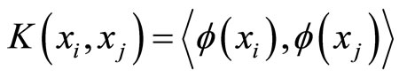
 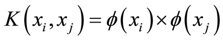 is the inner product kernel which satisfies Mercer’s condition [13] that is required for the generation of kernel functions given by:
 (5)
(5)
Thus, the support vectors associates with the desired outputs y(x) and with the input training data x can be defined by:
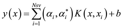 (6)
(6)
where xi are learning vectors. This leads to a SVM architecture (Figure 2) and are also founded in [2].
3.2.1. Kernel Functions
The use of an appropriate kernel is the key feature in support vector applications, since it provides the capability of mapping non-linear data into “feature” spaces that in essence are linear, then an optimization process can be applied as in the linear case. This provides a means to dimension the problem properly; nonetheless, the results still depend on the good selection of a set of training datasets.
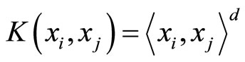
The Gaussian kernel function is defined in [11,30] Equation (7).
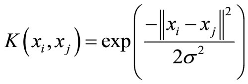 (7)
(7)
The Gaussian kernel process delivers an estimate for the reliability of the prediction in the form of the variance of the predictive distribution and the analysis can be used to estimate the evidence in favor of a particular choice of covariance function. The covariance or kernel function can be seen as a model of the data, thus providing a principled method for model selection [31,35].
A polynomial mapping is a widely used method for non-linear modeling [35], defined by:
 (8)
(8)
Unless the used of equation 8 implies an inherit problem, some support vector machines become zeros, therefore is preferable to rewrite the expression as:
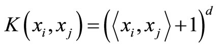 (9)
(9)
In this survey, a Spline kernel is presented as a choice for modeling due to their flexibility. A spline, of order with N knots located at ts is expressed by:
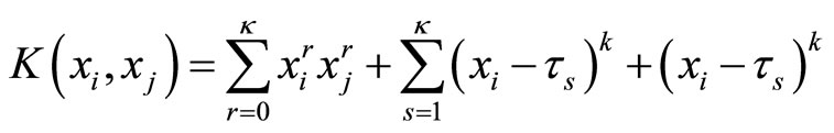 (10)
(10)
If k = 1 and the Spline function is defined as:
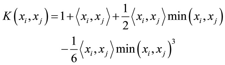 (11)
(11)
where the solution is a piecewise cubic.
3.2.2. Other Considerations
There are other considerations when working with SVMs on regression mode. The most important are: Bias Analysis, Free parameters and the quadratic problem. These issues will be discussed in this section.
The inclusion of a bias within the kernel function generally leads to a more efficient implementation and a slightly better accuracy model [11]. Conversely the solutions achieved with an implicit or explicit bias are not the same. This dichotomy emphasizes the difficulties whit
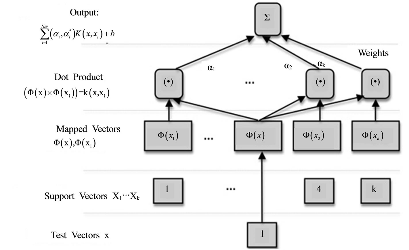
Figure 2. Support vector machine architecture.
the interpretation of generalization in high dimensional feature spaces. In this work the explicit bias approach is used.
Other important issue in support vector applications is the selection of free parameters such as the coefficient of C (regularization constant) and the value of error e. The regularization constant is the weight, determining the balance between the complexity of the network, while e is the margin within the error is neglected and in the Gaussian kernel function the value of variances s [11]. In previous contributions [35], it was found the optimum regularization coefficient to be 100 and the error e of 0.5.
In terms of the quadratic programming (QP), it becomes a problem when the number of data points exceeds a certain quantity (e.g. 2000). For SVM training with small data points works flawlessly [32,36].
In the study case of this survey, the number of data points is 365, where each data point represents the daily average of PMx concentration. Therefore the analysis and solving of the QP problem is not considered in the scope of this survey.
4. Proposed Methodology
The proposed Methodology has been taken from Lu [36] and Wang [37]. This methodology provides the general steps to make pollutants modeling and predictions by using SVM working in regression mode. In this survey Gaussian, Polynomial and Spline kernel functions are used. The aim of this work is to provide a natural representation of the system behavior, comparing the performance of the kernels used for this particular case study. In order to perform an appropriate design, training, and testing of SVM this article describes a generic methodology based on a review of [30,32], as shown in Figure 3.
The steps taken based on the methodology shown in Figure 1 are as follows:
Preprocessing of the input data by selecting the most relevant features, scaling the data in the range [−1, 1], and checking for possible outliers.
Selecting an appropriate kernel function that determines the hypothesis space of the decision and regression function.
Selecting the parameters of the kernel function, in polynomial kernels the degree for polynomials and the variances of the Gaussian kernels respectively.
Choosing the penalty factor C and the desired accuracy by defining the ε-insensitive loss function.
Validating the model obtained on some previously, during the training, unseen test data, and if not pleased iterate between steps “c” or, eventually “d”.
The fundamental reason for considering SVM working in regression mode as an approach for urban air pollution
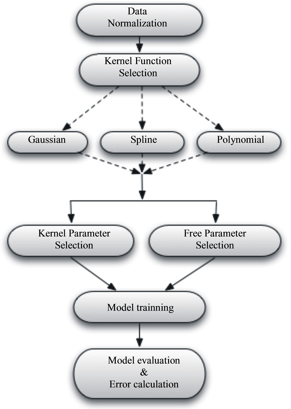
Figure 3. Proposed methodology.
modeling is the non-linear aspect of the application. There is no predetermined heuristic for the choice of free parameters and design for the SVM, many applications appear to be specific, in order to improve the SVM performance through the automatic adjustment of free parameters. Using SVM on real time applications appears to be rather complex due to the computational demands of the deriving results.
5. Experimental Results
Table 1 shows the forecasting results of Ozone considering all three kernels discussed in Section 3.2.1 for every month of the year. Here is shown the number of SVM used con construct the model for the specific kernel of the giving month. The bigger the number of SVM used, the bigger the computational cost to compute the model. Hence, the wanted accuracy (ratio of number of predicted and unpredicted points) has to be as high as possible keeping a small number of SVMs.
In this table, is shown that the number of support vector machines for the Gaussian kernel varies from 4 (February 2009) to 10 (December 2009). Although the accuracy is high for most predictions, it is worth noticing that both November and December has an accuracy far below the average (83.3% and 83.8, respectively) and the number of SVMs is also much higher than most of the other months, with the only exception for this for July. The best models with this kernel could be seen for February and June, where the accuracy is high (89.2% and 90%, respectively) maintaining a low computational cost with only 4 SVMs.
In terms of the polynomial kernel, the mode of number of kernels is between 5 and 6, with a lowest accuracy of 74.2% and the highest of 90.3 for some months. It is worth noting that it has a low accuracy (less than 80%) for the last three months of the year, a similar performance than the Gaussian kernel where the last months show a lower accuracy than the rest of the months. Furthermore, for the spline kernel, a low number of SMVs were needed to model Ozone and the accuracy varied from 67.7% (in December) to 93.5% (in March). In general, the lowest accuracy was shown for the last months of the year (especially December) for all three kernels. The kernel that shows a better steadiness was Gaussian for this particle, although for some months the number of SVMs was higher with its substantial increase of the computational cost. An example of a SVM forecasting for ozone using Gaussian kernel is shown in Figure 4.
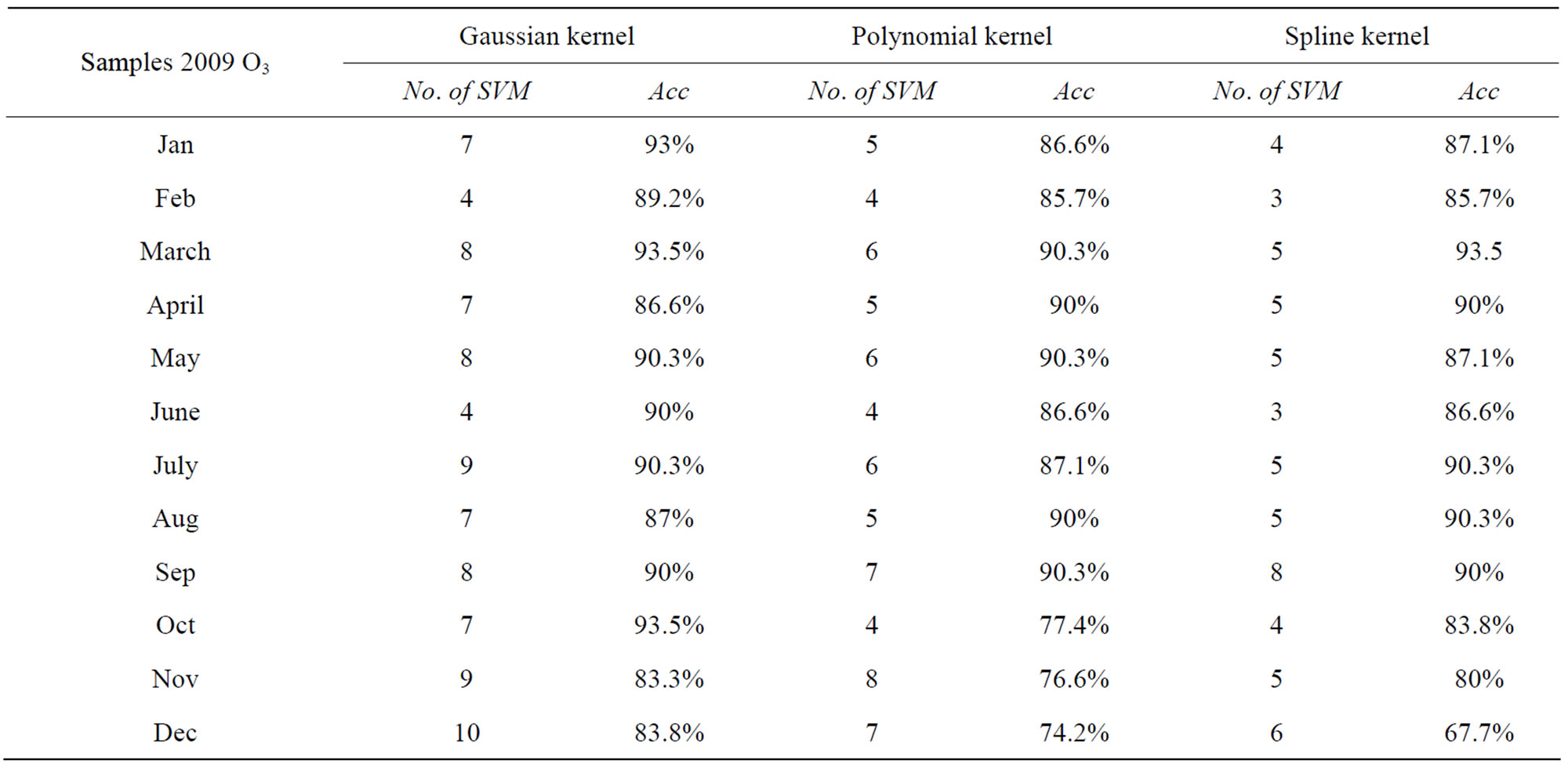
Table 1. Forecasting results ozone.
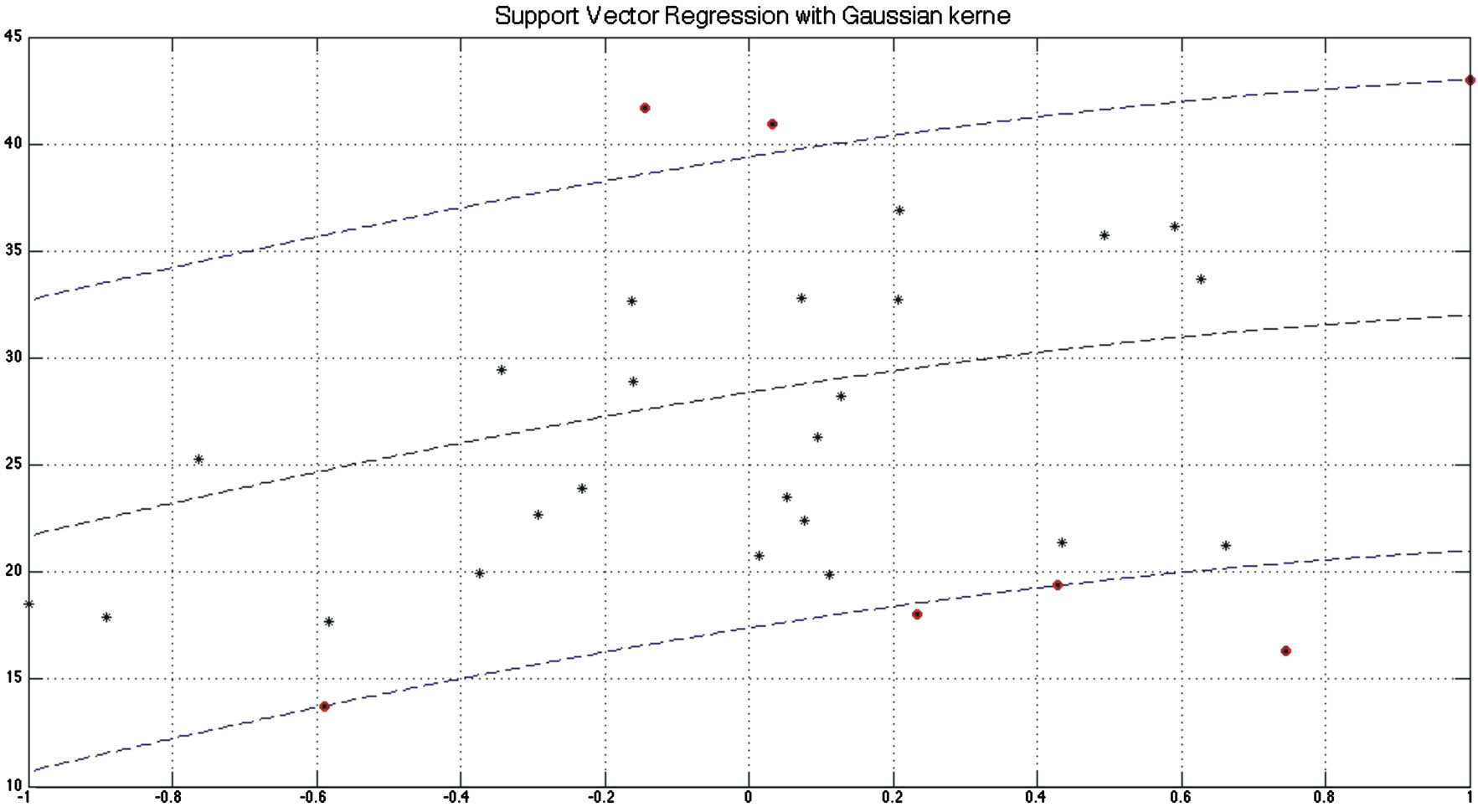
Figure 4. Forecasting of O3 concentration in January of 2009 using Gaussian kernel.
In Table 2 is shown the forecasting results for Nitrogen Dioxide for all three kernels. In this table, is shown that for this particle the highest accuracy is also for Gaussian kernel, which replicates the results for ozone. In general, the spline kernel shows the lowest number of SVMs to represent the model, but also the lowest accuracy in terms of percentage. An example of this behavior may be seen in Figure 5. Also, it can be noted that regardless of the kernel, the lowest accuracy for that specific kernel is located in the last months of the year (especially for December). This is also consistent with the forecasting results for ozone (Table 3).
In terms of the forecasting results for PM10, it can be noted that the Gaussian kernel works better in terms of accuracy in spite of the high number of SVMs to construct the model. Both spline and polynomial kernels work relatively accurate with a lower number of SVMs, with a few exceptions (e.g. Spline Kernel for April gives 10 SVMs with only 67.7% accuracy). An example of this behavior for spline kernel is shown in Figure 6.
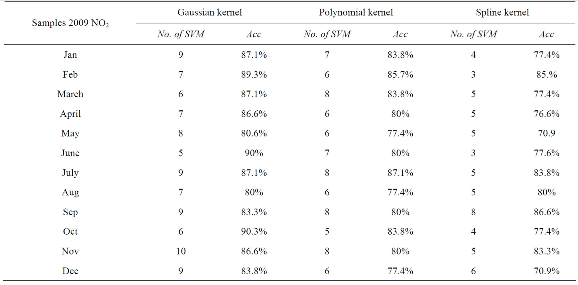
Table 2. Forecasting results nitrogen dioxide.
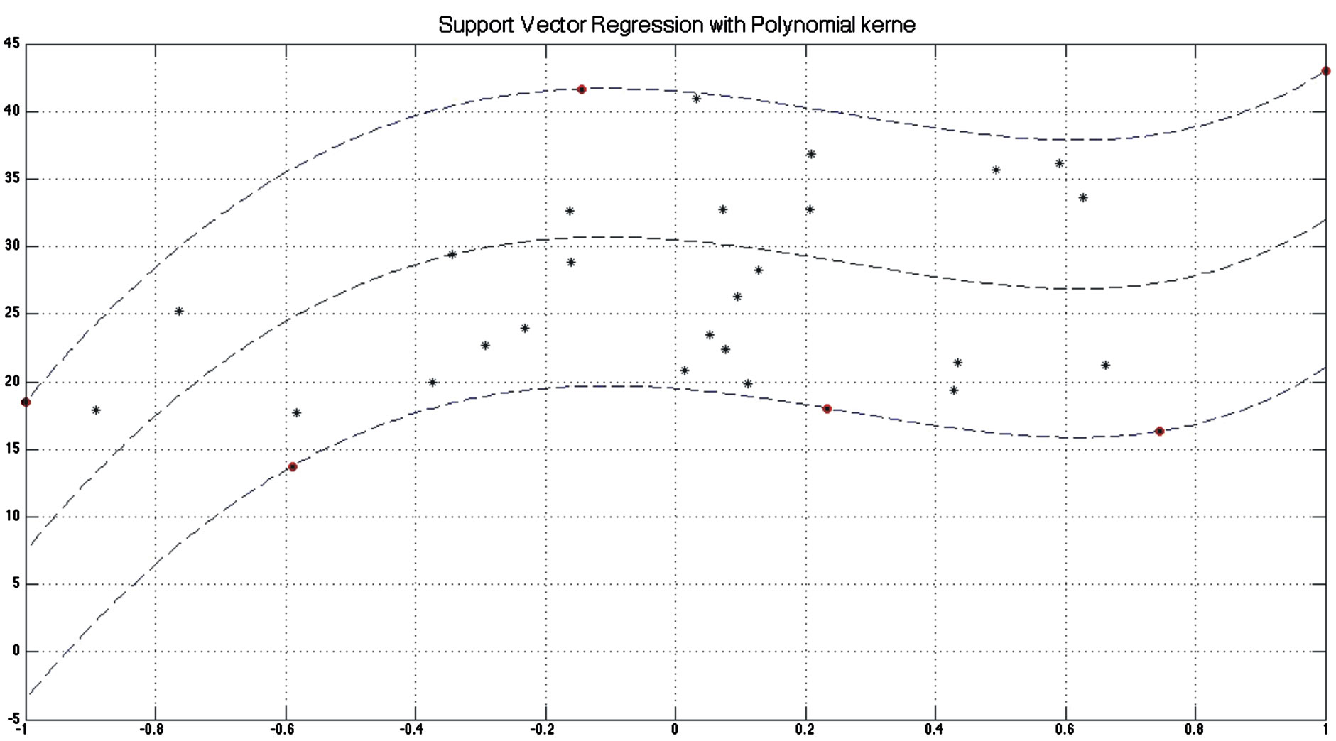
Figure 5. Forecasting of O3 concentration in January of 2009 using Polynomial kernel.
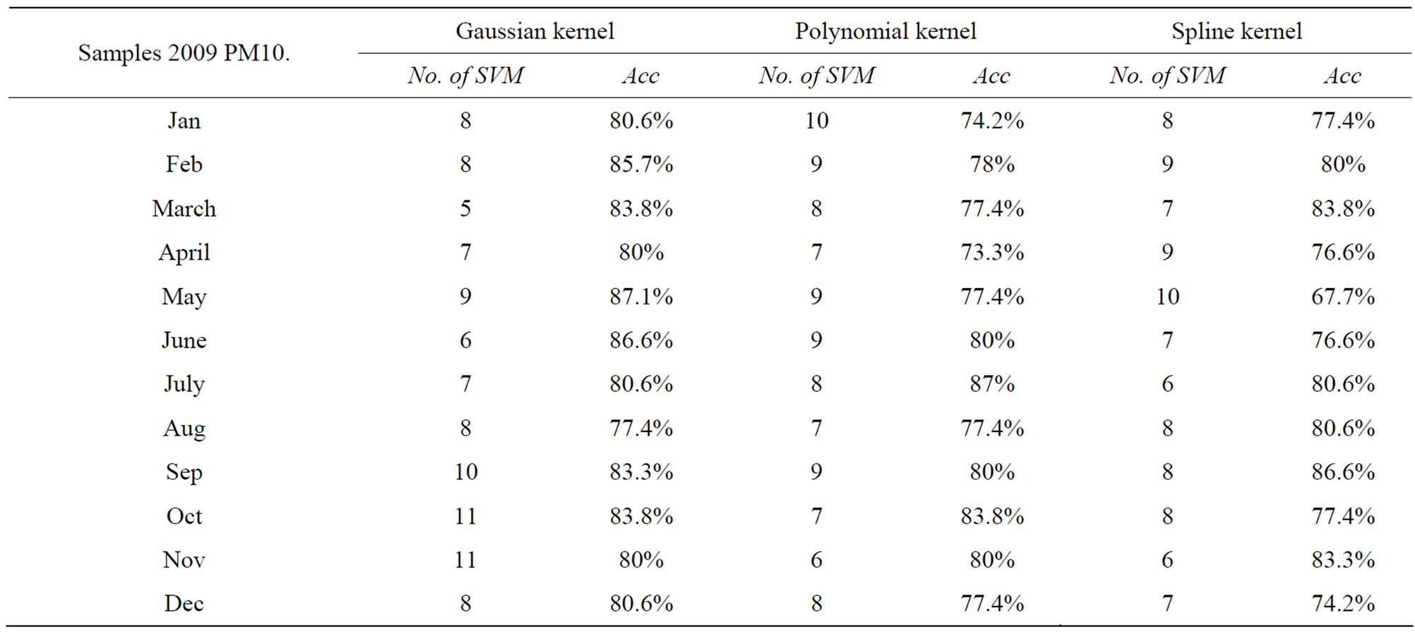
Table 3. Forecasting results PM10.
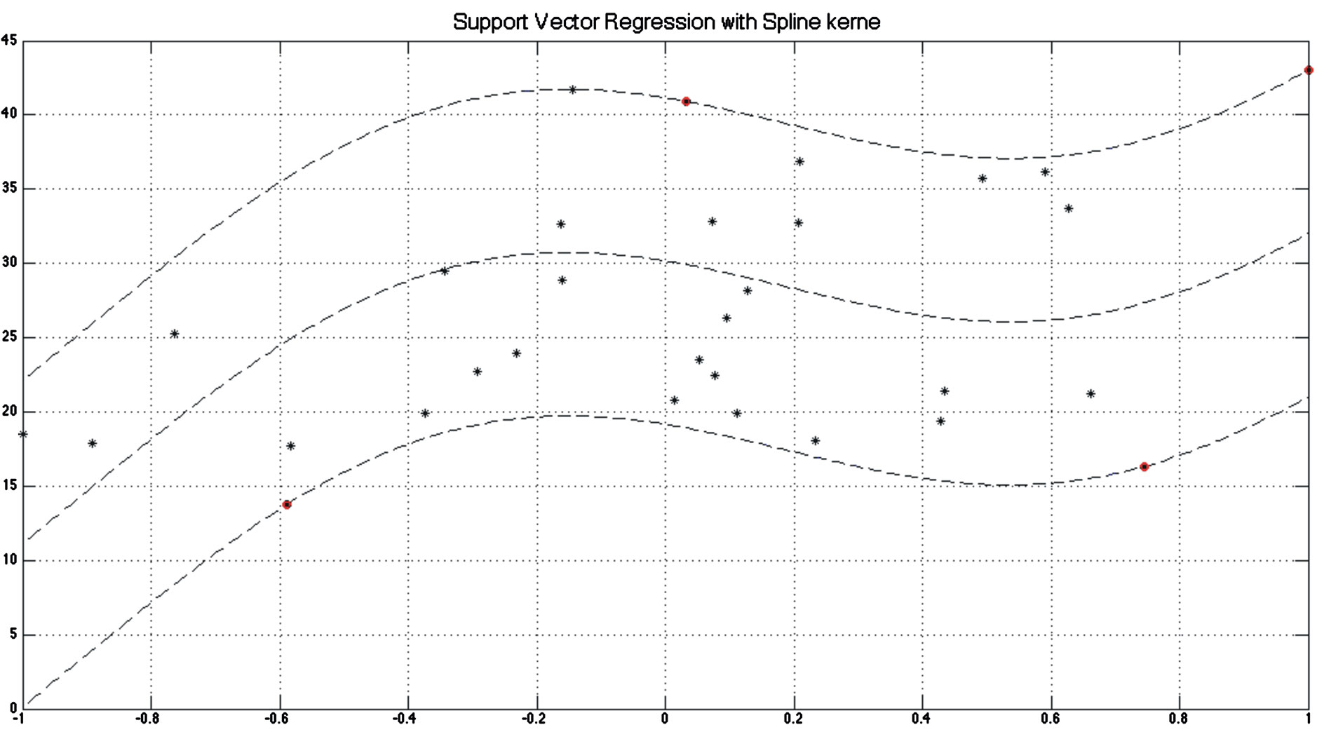
Figure 6. Forecasting of O3 concentration in January of 2009 using Spline kernel.
6. Conclusions and Future Work
This method presents a feasible modeling technique of the monthly atmospheric pollution by applying the support vector machine with Gaussian, Polynomial and Spline kernels functions working in regression mode. The application of SVM has enabled to obtain a good accuracy in modeling pollutant concentration of O3, NO2 and PM10 in Mexico City. The methods, techniques and alternatives offered in the SVM field provide a flexible and scalable tool for implementing sophisticated solutions with implied dynamical and non-linear data. It is noteworthy to point that the SVM guarantees this global minimum solution and a good feature of generalization.
Factors such as bias and free parameters were considered to construct the models. However, looking at the results, a trade-off must be made between computational cost in terms of number of support vector machines and accuracy. Looking at the results, it can be inferred that Gaussian kernel works better providing that the time to compute the results is not an issue. In general, Polynomial kernel does not offer an adequate performance in comparison with Gaussian for this particular case study.
As future work, implementing other kernel functions such as genetic, wavelet-based, principal component analysis (PCA), among others, may be considered for future contributions. Also a real-time prediction may be carried out using sensor networks and embedded systems.
REFERENCES
- E. Vega, E. Reyes and G. Sanchez, “Basic Statistics of PM2.5 and PM10 in the Atmosphere of Mexico City,” The Science of the Total Environment, Vol. 287, No. 3, 2002, pp. 167-176. doi:10.1016/S0048-9697(01)00980-9
- M. A. Aceves-Fernández, A. Sotomayor-Olmedo, E. Gorrostieta-Hurtado, J. C. Pedraza-Ortega, S. Tovar-Arriaga and J. M. Ramos-Arreguin, “Performance Assessment of Fuzzy Clustering Models Applied to Urban Airborne Pollution,” Proceedings of the 21st International Conference on Electrical Communications, San Andres Cholula, 28 February 2011-2 March 2011, pp. 212-216.
- M. Kolehmainen, H. Martikainen, T. Hiltunen and J. Ruuskanen, “Forecasting Air Quality Parameters Using Hybrid Neural Network Modeling,” Environmental Monitoring and Assessment, Vol. 65, No. 1-2, 2000, pp. 277- 286. doi:10.1023/A:1006498914708
- O. M. Pokrovsky, H. F. Roger and C. N. Kwok, “Fuzzy Logic Approach for Description of Meteorological Impacts on Urban Air Pollution Species: A Hong Kong Case Study,” Computers & Geosciences, Vol. 28, No. 1, 2002, pp. 119-127. doi:10.1016/S0098-3004(01)00020-6
- P. Viotti, G. Liuti and P. Di. Genova, “Atmospheric Urban Pollution: Applications of an Artificial Neural Network (ANN) to the City of Perugia,” Ecological Modelling, Vol. 148, No. 1, 2002, pp. 27-46. doi:10.1016/S0304-3800(01)00434-3
- C. Giorgio, “Air Quality Prediction in Milan: Feed-Forward Neural Networks, Pruned Neural Networks and Lazy Learning,” Ecological Modelling, Vol. 185, No. 2-4, 2005, pp. 513-529. doi:10.1016/j.ecolmodel.2005.01.008
- M. Caselli, L. Trizio, G. de Gennaro and P. Ielpo, “A Simple Feedforward Neural Network for the PM10 Forecasting: Comparison with a Radial Basis Function Network and a Multivariate Linear Regression Model,” Water, Air & Soil Pollution, Vol. 201, No. 1-4, 2009, pp. 365-377. doi:10.1007/s11270-008-9950-2
- K. P. Moustris, I. C. Ziomas and A. G. Paliatsos, “3-Day- Ahead Forecasting of Regional Pollution Index for the Pollutants NO2, CO, SO2, and O3 Using Artificial Neural Networks in Athens, Greece,” Water, Air & Soil Pollution, Vol. 209, No. 1-4, 2010, pp. 29-43. doi:10.1007/s11270-009-0179-5
- L. A. Diaz-Robles, J. C. Ortega, J. S. Fu, G. D. Reed, J. C. Chow, J. G. Watson and J. A. Moncada-Herrera, “A Hybrid ARIMA and Artificial Neural Networks Model to Forecast Particulate Matter in Urban Areas: The Case of Temuco, Chile,” Atmospheric Environment, Vol. 42, No. 35, 2008, pp. 8331-8340. doi:10.1016/j.atmosenv.2008.07.020
- M. M. Hossain, Md. R. Hassan and M. Kirley, “Forecasting Urban Air Pollution Using HMM-Fuzzy Model,” PAKDD’08 Proceedings of the 12th Pacific-Asia Conference on Advances in Knowledge Discovery and Data Mining, 20-23 May 2008, pp. 572-581.
- S. Osowski and K. Garanty, “Forecasting of the Daily Meteorological Pollution Using Wavelets and Support Vector Machine,” Engineering Applications of Artificial Intelligence, Vol. 20, No. 6, 2007, pp. 745-755. doi:10.1016/j.engappai.2006.10.008
- WHO (World Health Organization), “Environmental Burden of Disease,” No. 5, 2004.
- R. F. Phalen, “Introduction to Air Pollution Science: A Public Health Perspective,” 2012.
- J. H. Kilabuko, H. Matsuki and S. Nakai, “Air Quality and Acute Respiratory Illness in Biomass Fuel using homes in Bagamoyo, Tanzania,” International Journal of Environmental Research and Public Health, Vol. 4, No. 1, 2007, pp. 39-44. doi:10.3390/ijerph2007010007
- Y. L. Leo Lee, W.-H. Wang, C.-W. Lu, Y.-H. Lin and B.-F. Hwang, “Effects of Ambient Air Pollution on Pulmonary Function among Schoolchildren,” International Journal of Hygiene and Environmental Health, Vol. 214, No. 5, 2011, pp. 369-375. doi:10.1016/j.ijheh.2011.05.004
- D. Rao and W. Phipatanakul, “Impact of Environmental Controls on Childhood Asthma,” Current Allergy and Asthma Reports, Vol. 11, No. 5, 2011, pp. 414-420. doi:10.1007/s11882-011-0206-7
- H. H. Suh, A. Zanobetti, J. Schwartz and B. A. Coull, “Chemical Properties of Air Pollutants and Cause-Specific Hospital Admissions among the Elderly in Atlanta, Georgia,” Environmental Health Perspectives, Vol. 119, No. 10, 2011, pp. 1421-1428. doi:10.1289/ehp.1002646
- R. W. Boubel, D. L. Fox, D. B. Turner, A. C. Stern, “Fundamentals of Air Pollution,” 3rd Edition, Academic Press, Waltham, 1994.
- Achcar J. A., D. E. Fazioni Sousa, E. R. Rodrigues and T. Guadalupe, “Comparing the Number of Ozone Exceedances in Different Seasons of the Year in Mexico City,” Environmental Modeling and Assessment, Vol. 16, No. 3, 2011, pp. 251-264. doi:10.1007/s10666-010-9245-z
- J. Pey, A. Alastuey, X. Querol and S. Rodríguez, “Monitoring of Sources and Atmospheric Processes Controlling Air Quality in an Urban Mediterranean Environment,” Atmospheric Environment, Vol. 44, No. 38, 2010, pp. 4879-4890. doi:10.1016/j.atmosenv.2010.08.034
- M. R. O’Neill, D. Loomis and V. H. Borja-Aburto, “Ozone, Area Social Conditions and Mortality in Mexico City,” Environmental Research, Vol. 94, No. 3, 2004, pp. 234-242. doi:10.1016/j.envres.2003.07.002
- L. Emberson, M. Ashmore and F. Murray, “Air Pollution Impacts on Crops and Forests: A Global Assessment,” Imperial College Press, London, 2003.
- S. S. Ahmad, P. Biiker, L. Emberson and R. Shabbir, “Monitoring Nitrogen Dioxide Levels in Urban Areas in Rawalpindi, Pakistan,” Water, Air & Soil Pollution, Vol. 220, No. 1-4, 2011, pp. 141-150. doi:10.1007/s11270-011-0741-9
- H. Takizawa, “Impact of Air Pollution on Allergic Diseases,” The Korean Journal of Internal Medicine, Vol. 26, No. 3, 2011, pp. 262-273.
- M. Chiusolo, E. Cadum, M. Stafoggia, C. Galassi, G. Berti, A. Faustini, L. Bisanti, M. A. Vigotti, M. P. Dessì, A. Cernigliaro, S. Mallone, B. Pacelli, S. Minerba, L. Simonato and F. Forastiere, “Short-Term Effects of Nitrogen Dioxide on Mortality and Susceptibility Factors in 10 Italian Cities: The EpiAir Study,” Environmental Health Perspectives, Vol. 119, No. 9, 2011, pp. 1233-1238. doi:10.1289/ehp.1002904
- G. L. Peng, X. M.Wang, Z. Y.Wu, Z. M. Wang, L. L. Yang, L. J. Zhong and D. H. Chen, “Characteristics of Particulate Matter Pollution in the Pearl River Delta Region, China: An Observational-Based Analysis of Two Monitoring Sites,” Journal of Environmental Monitoring, Vol. 13, 2011, pp. 1927-1934. doi:10.1039/c0em00776e
- P. Lenschow, H. J. Abraham, K. Kutzner, M. Lutz, J. D. Preuß and W. Reichenbächer, “Some Ideas about the Sources of PM10,” Atmospheric Environment, Vol. 35, No. 1, 2001, pp. S23-S33. doi:10.1016/S1352-2310(01)00122-4
- A. L. Malcolm, R. G. Derwent and R. H. Maryon, “Modelling the Long-Range Transport of Secondary PM10 to the UK,” Atmospheric Environment, Vol. 34, No. 6, 2000, pp. 881-894. doi:10.1016/S1352-2310(99)00352-0
- J. X. Yin, R. M. Harrison, Q. Chen, A. Rutter and J. J. Schauer, “Source Apportionment of Fine Particles at Urban Background and Rural Sites in the UK Atmosphere,” Atmospheric Environment, Vol. 44, No. 6, 2010, pp. 841- 851. doi:10.1016/j.atmosenv.2009.11.026
- V. Vapnik, S. Golowich and A. Smola, “Support Method for Function Approximation Regression Estimation, and Signal Processing. Advances in Neural Information Processing Systems,” MIT Press, Cambridge, 1997.
- B. Schölkfopf, A. J. Smola and C. Burges, “Advances in Kernel Methods—Support Vector Learning, MIT Press, Cambridge, 1999.
- I. Sapankevych and R. Sankar, “Time Series Prediction Using Support Vector Machines: A Survey,” Computational Intelligence Magazine, Vol. 4, No. 2, 2009, pp. 24- 38. doi:10.1109/MCI.2009.932254
- E. Osuna, R. Freund and F. Girosi, “Support Vector Machines: Training and Applications,” Massachusetts Institute of Technology, Cambridge, 1997.
- N. Cristianini and J. Shawe-Taylor, “An Introduction to Support Vector Machines and Other Kernel-Based Learning Methods,” Cambridge University Press, Cambridge, 2000.
- A. Sotomayor-Olmedo, M. A. Aceves-Fernandez, E. Gorrostieta-Hurtado, J. C. Pedraza-Ortega, J. E. Vargas-Soto, J. M. Ramos-Arreguin and U. Villaseñor-Carillo, “Evaluating Trends of Airborne Contaminants by Using Support Vector Regression Techniques,” Proceedings of the 21st International Conference on Electrical Communications and Computers, San Andres Cholula, 28 February 2011-2 March 2011, pp. 137-141. doi:10.1109/CONIELECOMP.2011.5749350
- W. Lu and W. Wang, “Potential Assessment of the Support Vector Machine Method in Forecasting Ambient Air Pollutant Trends,” Chemosphere, Vol. 59, No. 5, 2005, pp. 693-701. doi:10.1016/j.chemosphere.2004.10.032
- F. Wang, D. S. Chen, S. Y. Cheng, J. B. Li, M. J. Li and Z. H. Ren, “Identification of Regional Atmospheric PM10 Transport Pathways Using HYSPLIT, MM5-CMAQ and Synoptic Pressure Pattern Analysis,” Environmental Modelling & Software, Vol. 25, No. 8, 2010 , pp. 927-934. doi:10.1016/j.envsoft.2010.02.004