Open Journal of Modern Hydrology
Vol.3 No.3(2013), Article ID:33990,13 pages DOI:10.4236/ojmh.2013.33014
Comparison of SCS and Green-Ampt Methods in Surface Runoff-Flooding Simulation for Klang Watershed in Malaysia
![]()
Faculty of Engineering, University of Nottingham Malaysia Campus, Kajang, Malaysia.
Email: kabiri.env@gmail.com
Copyright © 2013 Reza Kabiri et al. This is an open access article distributed under the Creative Commons Attribution License, which permits unrestricted use, distribution, and reproduction in any medium, provided the original work is properly cited.
Received January 4th, 2013; revised February 5th, 2013; accepted February 14th, 2013
Keywords: SCS Curve Number; Green-Ampt; Loss Method; GIS; HEC-Geo-HMS; HEC-HMS; Runoff; Flood Modeling
ABSTRACT
The main aim in this research is comparison the parameters of some storm events in the watershed using two loss models in Unit hydrograph method by HEC-HMS. SCS Curve Number and Green-Ampt methods by developing loss model as a major component in runoff and flood modeling. The study is conducted in the Kuala Lumpur watershed with 674 km2 area located in Klang basin in Malaysia. The catchment delineation is generated for the Klang watershed to get sub-watershed parameters by using HEC-GeoHMS extension in ARCGIS. Then all the necessary parameters are assigned to the models applied in this study to run the runoff and flood model. The results showed that there was no significant difference between the SCS-CN and Green-Ampt loss method applied in the Klang watershed. Estimated direct runoff and Peak discharge (r = 0.98) indicates a statistically positive correlations between the results of the study. And also it has been attempted to use objective functions in HEC-HMS (percent error peaks and percent error volume) to classify the methods. The selection of best method is on the base of considering least difference between the results of simulation to observed events in hydrographs so that it can address which model is suit for runoff-flood simulation in Klang watershed. Results showed that SCS CN and Green-Ampt methods, in three events by fitting with percent error in peak and percent error in volume had no significant difference.
1. Introduction
Usual methods of runoff and flooding estimation are costly, time consuming along with error because of having various variables contribute in the watershed. As such, using Geographic Information System (GIS), to develop hydrology model through the sub-watershed data in water resources management and planning seem to be critical. There are various methods to simulate surface runoff and flooding by using different loss model methods in HECHMS which some of them consist of the SCS Curve Number model [1], CASC2D [2], TOPMODEL [3], GIUH [4], University of British Columbia Watershed Model (UBCWM) and Geomorphological Instantaneous Unit Hydrograph (GIUH). Among the methods, the SCS (Natural Resources Conservation service Curve Number method (NRCS-CN)) method is widely used. Many studies have been conducted by [5-9] who have applied the GIS tools to estimate runoff CN value to make an empirical runoff estimation and also many researches was implemented by [10-13] to demonstrate SCS application in hydrological studies. This method is based on a rainfall-runoff model that was created to quantify direct runoff. In fact it presumes an initial abstraction according to curve number value. Curve numbers used in this study is according to USDA National Engineering Handbook [14]. To estimate the direct runoff (excess rainfall) the major components of a watershed which contribute to runoff are the data such as land use, soil data and antecedent moisture conditions (AMCs) which are designed to estimate the loss and runoff volume [15].
Green-Ampt is one of the other complicated methods which is assumed to better estimation of the impacts of land use on runoff. As stated by [16] infiltration parameters can be directly related to watershed characteristics. Green-Ampt method developed in 1911 which is an infiltration equation and requires the homogeneous soil characterizations such as hydraulic conductivity, wetting front soil suction head, moisture contents and impervious value. Some studies have been conducted on the performance of CN to Green-Ampt [17-19]. These studies demonstrate that results of direct runoff modeled are similar and state to be user friendly application of SCSCN method compare the Green-Ampt. Wilcox et al. (1990) expressed that CN and Green-Ampt models leave the results close to where the scope of the study was on six small catchments in USA.
In this study, SCS Curve Number and Green-Ampt equations are applied to determining loss model as a major component in runoff and flooding modeling. The objective of this study is to compare the results of SCS-CN and Green-Ampt model to estimate runoff and flooding in Klang watershed on some rainfall event data. It is important to mention that mapping watershed modeling is done using HEC-GeoHMS extension in ArcGIS which is able to produce the catchment delineation automatically and also acts as an interface between ArcGIS and HEC-HMS software.
2. Material
2.1. Study Area
This study was conducted in the Klang watershed, located in Kuala Lumpur, Selangor province in Malaysia given in Figure 1. The scope lies between 101˚30' to 101˚55' E Longitudes and 3˚N to 3˚30'N latitude. The area of Klang watershed is approximately 674 km2. The elevation ranges from 10 to 1400 meter above mean sea level and the mean annual precipitation is about 2400 mm. About 50% of Klang watershed has occupied by urban area and much of it is perched on susceptible land to flooding. The Figures 2 and 3 illustrate the major landuses and soil in the study area respectively. Table 1 address most cover types that are commonly encountered in Klang watershed areas.

Figure 1. Location of the study area.
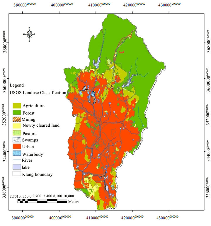
Figure 2. Land use/cover map of the Klang watershed.

Figure 3. Soil map of the Klang watershed.
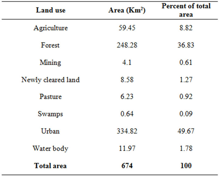
Table 1. Land use/cover classes present in the Klang watershed (from DID, 2002).
2.2. Data Sources
The Landuse, Soil, rainfall data and hydrometric data (Hourly discharge) were obtained from Department of Irrigation and Drainage of Malaysia (DID). Digital Elevation Model (DEM) obtained from the Shuttle Radar Topography Mission (SRTM) with the resolution of 90 meters per pixel. 18 rainfall gage stations were selected in the scope of study which contributes to process of areal rainfall mapping. The Table 2 given the geographical coordination of 18 rainfall gage stations located in the study area. Figure 1 shows the spatial map of all the rainfall station.
2.3. Software Used for Data Processing
ArcGIS version 9.3.1 powerful Geographical Information System (GIS) software with the HEC-GeoHMS extension used for creating hydrological maps. The extension is a hydrological tool developed by US Army Corps of Engineers, Hydrologic Engineering Center, 2003 and also HEC-HMS software is used for Runoff and flooding analysis.
3. Methodology
According to the Figure 4, there has been created catchment delineation for the Klang watershed to make the sub-watershed parameters by using HEC-GeoHMS extension in ARCGIS as an input into HEC-HMS. In this regard, there has been attempt to reproduce all the spatial maps such as initial content, saturated content, suction and conductivity maps extracted from soil data for Green-Ampt method and also other necessary maps for SCS-CN method such as Hydrological soil groups (HSGs), CN and initial abstraction maps. In addition, spatial impervious map developed by overlaying the DEM and landuse map by cross function in ArcGIS. To enter the precipitation data in HEC-HMS for each subwatershed, there has been made an aerial rainfall data interpolation for the rainfall event used in the modeling using geostatistical extension in ArcGIS. Since the landuse map in this study is devoted to 2002, therefore relevant flood events are extracted from the year of 2002. The rainfall events with the simple hydrograph shape selected which seem to be appropriate in runoff-flooding modeling by HEC-HMS. The events of 11 June and 21 Dec. are used for validation. Muskingum method is run and finally Muskingum method has been run to enter the channel haracterization for flood hydrograph setup in HEC-HMS.
To add the point, that there are two reservoirs in Klang watershed (Batu dam and Klang gate dam). According to its characterization a storage-discharge relationship was run in HEC-HMS to determine the detention impact of the reservoirs.
3.1. Loss Model to Determine Excess Precipitation (Direct Runoff)
3.1.1. SCS-Curve Number Method
The SCS-CN method is used in runoff volume calculation using the values related to landuse and soil data so that integration of these data determine CN values for the watershed to consider amount of infiltration rates of soils. The CN values for all the types of land uses and hydrologic soil groups in Klang watershed are adopted from Technical Release 55 [14]. In this regard, Soils are categorized into hydrologic soil groups (HSGs). The HSGs consist of four categories A, B, C and D, which A and D is the highest and the lowest infiltration rate respectively. To create the CN map, the hydrologic soil group and land use maps of the Klang watershed are combined by cross function in ARCGIS to get a new map integrated of both the land use and soil data.
3.1.2. Green-Ampt Method
Green and Ampt method is also used to calculate the infiltration and loss rate in runoff modeling. The Green Ampt Method is an acceptable loss model and is a simplified representation of the infiltration process in the field [20]. It is a function of the soil suction head, porosity, hydraulic conductivity and time. The general formula of Green-Ampt method is given below [21].
 (1)
(1)
where, F is the total depth of infiltration. Ψ is wetting front soil suction head, θ is water content in terms of volume ratio and K is a saturated hydraulic conductivity.
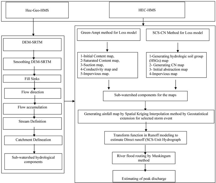
Figure 4. Flowdiagram of flood modeling using Hec-Geo-HMS.
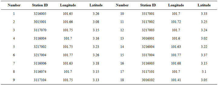
Table 2. Rainfall station used in the study.
The soil texture is important component due to it impacts soil physical properties which are used in GreenAmpt method to calculate the loss parameters. In order to estimate soil properties in the Kland watershed it is categorized into USDA soil texture classification. Therefore, the values suggested by [22] have been adapted in soil characterizations.
3.2. SCS-Unit Hydrograph
The curve of runoff changes in terms of time is called hydrograph. It is able to prepare the maximum runoff, volume and the amount of retention of flooding in a watershed. In this study, SCS Dimensionless Hydrograph has been used to generate unit hydrograph for the selected event rainfall. This method has been by USDA on the various watersheds in US. It based on the converting time and flow axis to dimensionless hydrograph in flood hydrograph. It is implemented by dividing the real time of hydrograph by “time to peak”, and also dividing the flow of hydrograph by “flow to peak. The method is based on the two assumptions which state firstly, flow at any time is proportional to the volume of runoff, and secondly, time factors affecting the hydrograph shape are constant [14]. The parameters used in SCS dimensionless unit hydrograph are Time of concentration, Lag time, Duration of the excess Rainfall, Time to peak flow, Peak flow. The relevant equations listed below:
 (2)
(2)
 (3)
(3)
 (4)
(4)
where, Q is direct runoff (mm), P is accumulated rainfall (mm), S is potential maximum soil retention (mm), and CN is Curve Number.
The unit hydrograph for any regularly shaped watershed can be constructed once the values of Qp and Tp are defined. The time to peak, time of concentration and is defined as:
 (5)
(5)
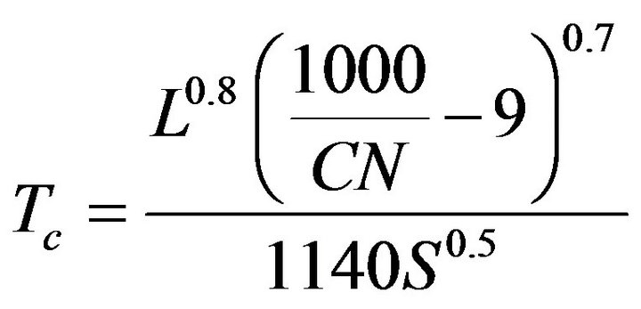 (6)
(6)
 (7)
(7)
where, Tp is Time to peak (min), Tc is Time of concentration (hr.), L is hydraulic length of watershed (ft), S is average land slope of the watershed (percent), qp is peak flow , Q is direct runoff (cm), A is area of watershed (Km2). tp is Time to peak (hr.)
The standard lag time is defined as the length of time between the centroid of precipitation mass and the peak flow of the hydrograph. The time of concentration is defined as the length of time between the ending of excess precipitation and the first milestone on descending hydrograph.
3.3. Flow Calculation in Reach
There are some methods to consider the flow hydrograph in HEC-HMS. According the available data of the Klang watershed, Muskingum method is run to determine the effect of detention of the river on flood hydrograph. Reach element conceptually represents a segment of stream or river. The general formula of Muskingum developed by US Army Corps of Engineers.
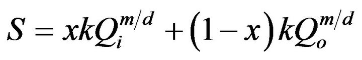 (8)
(8)
where, S is the amount of storage , Qi and Qo is inflow and outflow
 , m and d are the constant values which express the logarithmic relationship between storage and elevation.
K is called to storage coefficient having dimensions of time and expressing the ratio of storage to outflow level and can be considered as travel time through the reach element. X is a constant coefficient specifying the relative influence of inflow (Qi) and outflow (Qo) levels which ranges from 0.0 up to 0.5 with a value of 0 results in maximum attenuation and 0.5 results in no attenuation (HEC-HMS tutorial). In this study due to having the most urbanization areas occupied in Klang watershed, value of coefficients has been taken as 0.5.
4. Results and Discussion
4.1. Generating Hydrological Watershed Characterization
Once downloading the DEM from SRTM site, it is run some processes on it to generate the sub-watersheds and relevant hydrological characterization. The smoothing and filling function are applied by HEC-Geo-HMS to remove the null and noise of DEM. Flow direction, flow accumulation and stream definition functions are run to reproduce the drainage network of DEM. Finally “catchment delineation” function in HEC-Geo-HMS generated 33 sub-watersheds. The Figure 5 displays generated sub-watersheds and Table 3 presents morphological characterization of Klang watershed derived from DEM.
4.2. Generating HGSs and CN Maps
Three hydrologic groups including A, B and D were found in the Klang watershed. 32, 11.6 and 55.5 percent of soil placed in group A, B and D, respectively. Figure 6 illustrates CN map. And also Table 4 presents CN values obtained by overlaying the land use and soil maps. It is founded that the lowest CN value was found to be 30 in forest and industrial area with the highest CN value was found to be 93 (except the water body which CN equal to 100).
Next step is to make average for each sub-watershed which has been delineated already. The GIS Cross function is employed to generate sub-watershed CN and Green-Ampt maps using Equation (9):
 (9)
(9)
where:  is weighted average soil parameter for sub-watershed;
  is the parameter value and
  is area inside the specified sub-watershed.
All the values assigned to sub-watershed in Klang area are presented in Table 5.
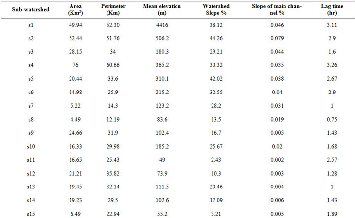
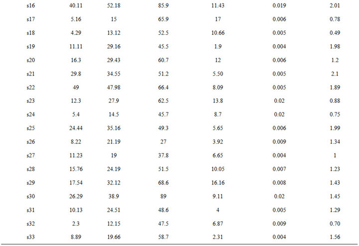
Table 3. Sub-watershed parameters derived of Klang watershed.
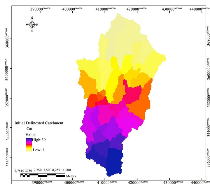
Figure 5. Sub-watershed derived of the Klang watershed.
Figure 6. Map of curve number (CN) values for Klang watershed.

Table 4. Curve number of different land use and Hydrologic soil groups (HSGs) in Klang watershed.
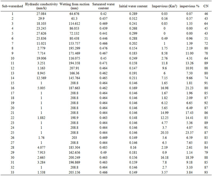
Table 5. Infiltration parameters in Green-Ampt method for each sub-watershed in Klang area.
4.3. Generating Green-Ampt Maps
Green-Ampt has essential parameters for flood-runoff modeling. To make Green-Ampt parameters at first all the relevant infiltration values adapted from Rawls and Brakensiek (1983) were assigned into soil texture map in GIS. And then it is attempted to make an average value of the infiltration parameters according to sub-watershed boundary by HEC-Geo-HMS to estimate the loss model maps such as hydraulic conductivity, suction and initial maps and also the percentage of impervious map. Figure 7 is hydraulic conductivity map as an illustration of Green-Ampt component. Table 5 presents all the GreenAmpt parameters for each sub-basin.
4.4. Generating Direct Runoff and Peak Discharge
Once all the parameters were setup in HEC-HMS for the both loss models (SCS-CN and Green-Ampt), the models run to obtain the direct runoff and peak discharge for each sub-watershed. Table 6 displays the output of models run according to flood event of 6 May 2002.
5. Conclusion
In order to determine the efficiency and suitability of methods used there has been attempted to make a comparison on the results by some correlation coefficients and error indices such as Mean Square Error (RMSE), Mean Absolute Error (MAE), coefficient of determination (R2), correlation coefficient (r), Nash-Sutcliffe efficiency (NSE) where as RMSE and MAE values of 0 indicate a perfect fit. R2, r and NSE values of 1 indicate perfect correlation. Model for each methods run and the results are presented in Table 6. A comparison is conducted on the results of Green & Ampt to SCS-CN loss methods for estimation of runoff losses (Table 7). And also the selection of best method is on the base of considering least difference between the results of simulation to observed events in hydrographs so that it can address which model is suit for runoff-flood simulation in Klang watershed (Table 8). The comparison indicates that the
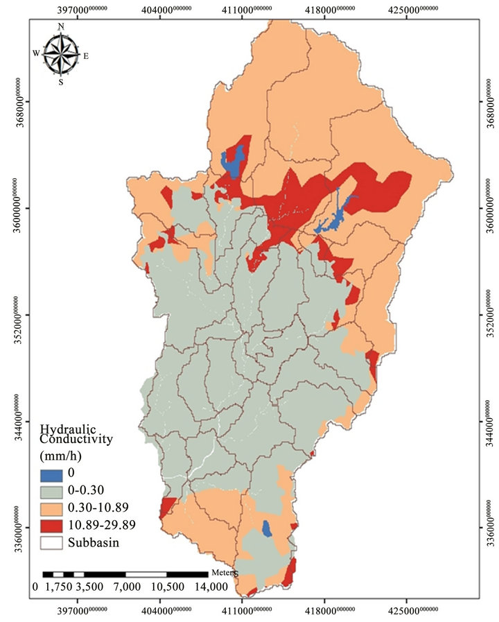
Figure 7. Hydraulic conductivity map of Klang watershed.

Table 6. The comparison of peak discharge and total direct runoff modeled by SCS-CN and Green-Ampt loss methods in HEC-HMS for each sub-watershed in Klang area.
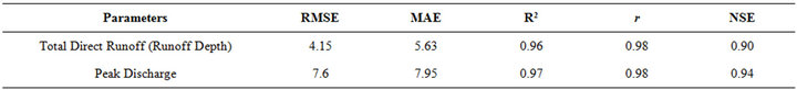
Table 7. Evaluation of Green-Ampt and SCS-CN methods for calculating total direct runoff and peak discharge.
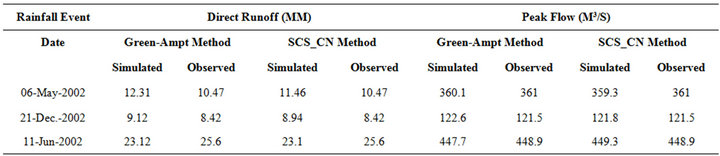
Table 8. The comparison of direct runoff and peak discharge by use of objective functions.
Green-Ampt and SCS-CN loss methods in three events have no significant difference in results of runoff and flood studies in Klang watershed.
REFERENCES
- USDA-SCS, “National Engineering Handbook, Section 4-Hydrology,” USDA-SCS, Washington DC, 1985.
- M. Marsik and P. Waylen, “An Application of the Distributed Hydrologic Model CASC2D to a Tropical Montane Watershed,” Journal of Hydrology, Vol. 330, No. 3-4, 2006, pp. 481-495.
- K. Warrach, M. Stieglitz, H. T. Mengelkamp and E. Raschke, “Advantages of a Topographically Controlled Runoff Simulation in a Soil-Vegetation-Atmosphere Transfer Model,” Journal of Hydrometeorology, Vol. 3, No. 2, 2002, pp. 131-148. doi:10.1175/1525-7541(2002)003<0131:AOATCR>2.0.CO;2
- R. Kumar, C. Chatterjee, R. D. Singh, A. K. Lohani and S. Kumar, “Runoff Estimation for an Ungauged Catchment Using Geomorphological Instantaneous Unit Hydrograph (GIUH) Model,” Hydrological Process, Vol. 21, No. 14, 2007, pp. 1829-1840. doi:10.1002/hyp.6318
- A. Pandey and A. K. Sahu, “Generation of Curve Number Using Remote Sensing and Geographic Information System,” 2002. http://www.GISdevelopment.net
- T. R. Nayak and R. K. Jaiswal, “Rainfall-Runoff Modelling Using Satellite Data and GIS for Bebas River in Madhya Pradesh,” Journal of the Institution of Engineers, Vol. 84, 2003, pp. 47-50.
- X. Zhan and M. L. Huang, “ArcCN-Runoff: An ArcGIS Tool for Generating Curve Number and Runoff Maps,” Environmental Modelling and Software, Vol. 19, No. 10, 2004, pp. 875-879. doi:10.1016/j.envsoft.2004.03.001
- M. L. Gandini and E. J. Usunoff, “SCS Curve Number Estimation Using Remote Sensing NDVI in a GIS Environment,” Journal of Environmental Hydrology, Vol. 12, 2004, p. 16.
- G. De Winnaar, G. Jewitt and M. Horan, “GIS-Based Approach for Identifying Potential Runoff Harvesting Sites in the Thukela River Basin, South Africa,” Physics and Chemistry of the Earth, Vol. 32, 2007, pp. 1058-1067. doi:10.1016/j.pce.2007.07.009
- C. Michel, A. Vazken and C. Perrin, “Soil Conservation Service Curve Number Method: How to Mend a Wrong Soil Moisture Accounting Procedure,” Water Resources Research, Vol. 41, No. 2, 2005, pp. 1-6.
- L. E. Schneider and R. H. McCuen, “Statistical Guidelines for Curve Number Generation,” Journal of Irrigation and Drainage Engineering, Vol. 131, No. 3, 2005, pp. 282-290.
- S. Mishra, R. Sahu, T. Eldho and M. Jain, “An Improved IaS Relation Incorporating Antecedent Moisture in SCSCN Methodology,” Water Resources Management, Vol. 20, No. 5, 2006, pp. 643-660. doi:10.1007/s11269-005-9000-4
- R. K. Sahu, S. K. Mishra, T. I., Eldho and M. K., Jain, “An Advanced Soil Moisture Accounting Procedure for SCS Curve Number Method,” Hydrological Processes, Vol. 21, No. 21, 2007, pp. 2872-2881. doi:10.1002/hyp.6503
- US Department Agriculture, Soil Conservation Service, “Urban Hydrology for Small Watersheds SCS Technical Release 55,” US Government Printing Office, Washington DC, 1986.
- S. K. Mishra, M. K. Jain, R. P. Pandey and V. P. Singh, “Catchment Area-Based Evaluation of the AMC-Dependent SCS-CN-Inspired Rainfall-Runoff Models,” Journal of Hydrological Process, Vol. 19, No. 14, 2005, pp. 2701- 2718. doi:10.1002/hyp.5736
- B. P. Wilcox, W. J. Rawls, D. L Brakensiek and J. R. Wight, “Predicting Runoff from Rangeland Catchments: A Comparison of Two Models,” Water Resources Research, Vol. 26, No. 10, 1990, pp. 2401-2410.
- X. C. Zhang, M. A. Nearing and L. M. Risse, “Estimation of Green-Ampt Conductivity Parameters: Part I. Row Crops,” Transactions of the ASAE, Vol. 38, No. 4, 1995, pp. 1069-1077.
- X. C. Zhang, M. A. Nearing and L. M. Risse, “Estimation of Green-Ampt Conductivity Parameters: Part II. Perennial Crops,” Transactions of the ASAE, Vol. 38, No. 4, 1995, pp. 1079-1087.
- M. A. Nearing, B. Y. Liu, L. M. Risse and X. Zhang, “Curve Numbers and Green-Ampt Effective Hydraulic Conductivities,” Journal of the American Water Resources Association, Vol. 32, No. 1, 1996, pp. 125-136. doi:10.1111/j.1752-1688.1996.tb03440.x
- S. T. Chu, “Infiltration during Unsteady Rain,” Water Resources Research, Vol. 14, No. 3, 1970, pp. 461-466.
- R. G. Mein and C. L. Larson, “Modeling Infiltration during a Steady Rain,” Water Resources Research, Vol. 9, No. 2, 1973, pp. 384-394. doi:10.1029/WR009i002p00384
- W. J. Rawls and D. L. Brakensiek, “A Procedure to Predict Green and Ampt Infiltration Parameters,” Proceedings of the National Conference on Advances in Infiltration Chicago, Chicago, 1983, pp. 12-13.