Open Journal of Modern Hydrology
Vol. 2 No. 4 (2012) , Article ID: 23416 , 12 pages DOI:10.4236/ojmh.2012.24010
Conditional Heteroscedasticity in Streamflow Process: Paradox or Reality?
![]()
Department of Agricultural & Bioresources Engineering, Federal University of Technology, Minna, Nigeria.
Email: martynso_pm@yahoo.co.uk, martynso_pm@futminna.edu.ng
Received June 26th, 2012; revised August 1st, 2012; accepted August 28th, 2012
Keywords: Autoregressive; Homoscedasticity; Volatility; Nonlinear Dynamics
ABSTRACT
The various physical mechanisms governing the dynamics of streamflow processes act on a seemingly wide range of temporal and spatial scales; almost all the mechanisms involved present some degree of nonlinearity. Against the backdrop of these issues, in this paper, attempt was made to critically look at the subject of Autoregressive Conditional Heteroscedasticity (ARCH) or volatility of streamflow processes, a form of nonlinear phenomena. Towards this end, streamflow data (both daily and monthly) of the River Benue, Nigeria were used for the study. Results obtained from the analyses indicate that the existence of conditional heteroscedasticity in streamflow processes is no paradox. Too, ARCH effect is caused by seasonal variation in the variance for monthly flows and could partly explain same in the daily streamflow. It was also evident that the traditional seasonal Autoregressive Moving Average (ARMA) models are inadequate in describing ARCH effect in daily streamflow process though, robust for monthly streamflow; and can be removed if proper deseasonalisation pre-processing was done. Considering the findings, the potential for a hybrid Autoregressive Moving Average (ARMA) and Generalised Autoregressive Conditional Heteroscedasticity (GARCH)- type models should be further explored and probably embraced for modelling daily streamflow regime in view of the relevance of statistical modelling in hydrology.
1. Introduction
When modelling hydrologic time series, the focus usually is on modelling and predicting the mean behaviour, or the first order moments, and rarely, is it concerned with the conditional variance, or their second order moments; although unconditional season-dependent variances are usually considered. The increased importance played by risk and uncertainty considerations in water resources management and flood control practice, as well as in modern hydrology theory, however, has necessitated the development of new time series techniques that allow for the modelling of time varying variances. It is not hard to find evidence to argue that a time series with random appearance might be nonlinear dynamic; but it suffices to note that the difficulty is in telling what kind of nonlinear dynamics.
To a large extent, one can think of heteroscedasticity as time-varying variance (i.e., volatility); in this regard, a univariate stochastic process is said to be homoscedastic if variances of the time series are constant. The “conditional” term as used in the definition of Autoregressive Conditional Heteroscedasticity (ARCH) or Generalised Autoregressive Conditional Heteroscedasticity (GARCH)-type models, implies a dependence on the observations of the immediate past, while autoregressive describes a feedback mechanism that incorporates past observations into the present. Thus, GARCH can be described as a mechanism that includes past variances in the explanation of future variances. It allows users to model the serial dependence of volatility, as it takes into account excess kurtosis (i.e., fat tail behaviour), which is very common in hydrologic processes, and volatility clustering. Volatility clustering as used here depicts a phenomenon in which large changes tend to follow large changes, and small changes tend to follow small changes. In either of these cases, the changes from one period to the next are typically of unpredictable sign or orientation. Basically, the concept of volatility suggests a time-series model in which successive disturbances, although uncorrelated, are nonetheless serially dependent. A time series with the ARCH property has two basic components: conditional mean, and a conditional variance function; thus, the nonlinearity in the series may probably come from the nonlinearity of the conditional variance.
ARCH-type models can generate accurate forecasts of future volatility, especially over short horizons, therefore providing a better estimate of the forecast uncertainty which is available for water resource management and flood control [1]; as such, ARCH-type models could be very useful for hydrologic time series modelling. Some proposals on new models [2] to reproduce the asymmetric periodic behaviour with large fluctuations around large streamflow and small fluctuations around small streamflow are available. These fluctuations though, basically can be handled with the conventional time series models that take season-dependent variance into account, such as Periodic Autoregressive Moving Average (PARMA) models and deseasonalised Autoregressive Moving Average (ARMA) models. However, little attention has been paid so far by the hydrologic community to test and model the possible presence of the ARCH effect with which large fluctuations tend to follow large fluctuations, and small fluctuations tend to follow small fluctuations in streamflow series [1]. Besides the recognised physical sources, such as the mechanisms involved in the rainfall-runoff transformation, some other sources can be identified from the streamflow series itself; for instance, issues of heteroscedasticity or volatility, nonlinear deterministic chaos and fractals. In this regard therefore, it is imperative to realise that both conditional heteroscedasticity and asymmetric seasonality in the mean and variance could also be probable sources of nonlinearity within the overall context of nonlinear determinism itself [1,3,4].
Against the backdrop of all this, the objective of this study, patterned after Wang et al. [1], is to test for the existence of ARCH effect in both the daily and monthly streamflow series of the River Benue, Nigeria. In addition, if there is the existence of ARCH effect, propose an ARMA-GARCH error model for the daily streamflow series since the ARCH theory admits non-normality of the unconditional distribution of the data. Thus, with the assumption of normality of the conditional distribution, an ARCH-type structure could be built to capture the time-dependent variances. The idea to restrict the modelling exercise to a low timescale is because of the short length of the monthly series.
2. Materials and Methods
2.1. Data Base
In this study, historical time series for gauging stations at the base of the River Benue (i.e., Lower Benue River Basin) at Makurdi (7˚44' N, 8˚32' E), Nigeria was used. A total of 26 years (1974-2000) water stage and daily discharge data were collected. The average daily discharges were then aggregated to monthly discharge values; both data regimes were used as appropriate in the study. To achieve this, discharge rating curve was used to convert the stage data to the corresponding discharge values. Figure 1 below shows the Benue River and its traverse; indicated too, is the study location, i.e., Makurdi.
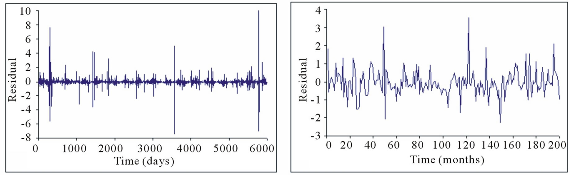
Both Figures 2 and 3 show the irregular flow pattern of the streamflow processes; i.e., daily and monthly time resolutions. The irregular flow pattern derives from the implications of seasonality. The study area experiences two distinct seasons, the wet and dry seasons respectively. Because seasonality impacts greatly on the behavioural pattern of flow vis-a-vis anthropogenic factors, prior to model development, data pre-processing was done as reported in the later sections of the study.
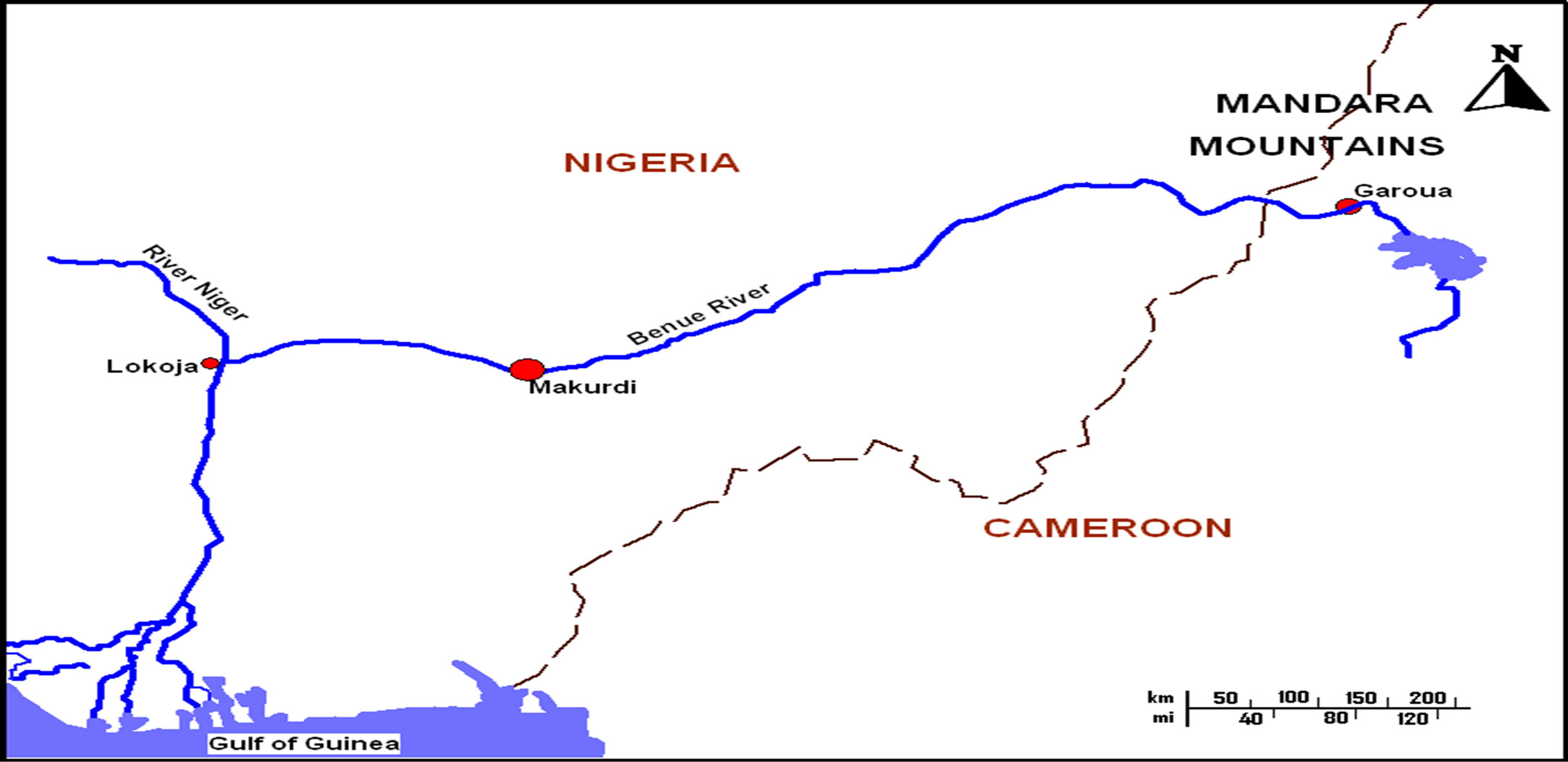
Figure 1. Map of Nigeria showing the River Benue and the study location.
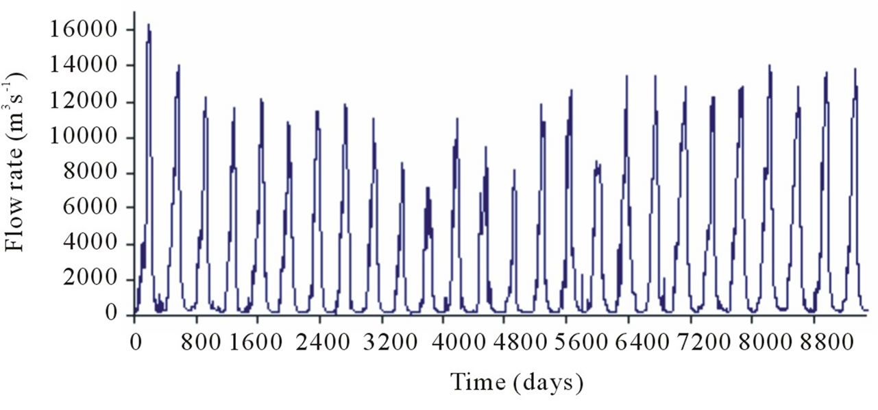
Figure 2. Time series plot of the daily streamflow.
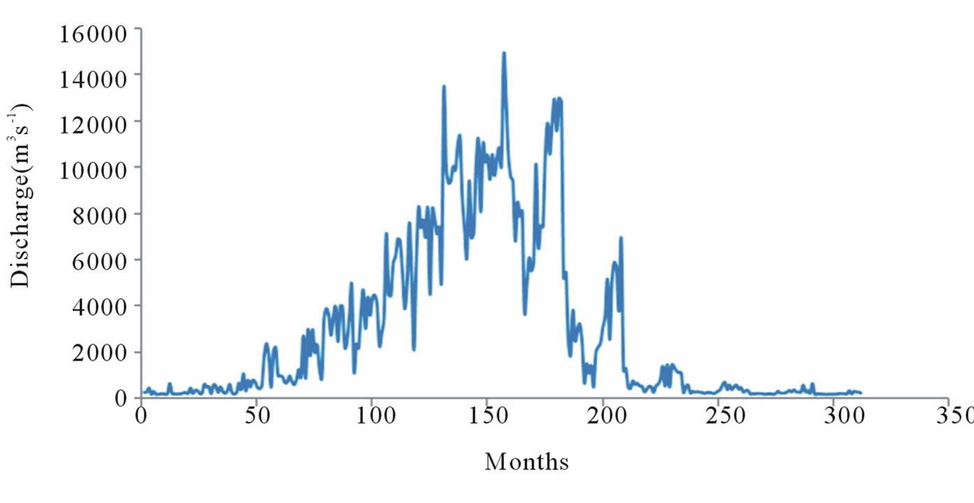
Figure 3. Monthly discharge series plot.
2.2. Tests for ARCH Effect
The detection for the ARCH effect of a streamflow series is actually a test of serial independence applied to the serially uncorrelated fitting error of some model, usually a linear stochastic autoregressive (AR) model. Suppose a stochastic process Yt is generated by an AR(p) process:
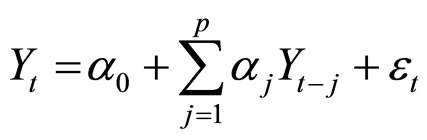 (1)
(1)
There exists an information set  such that:
 (2)
(2)
where
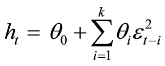 (3)
(3)
with
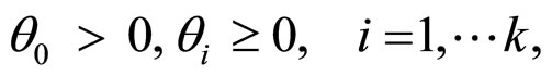 (4)
(4)
to ensure, that the conditional variance is positive. The process Yt is called AR(p) with ARCH(k) errors. It is important to note that the conditional variance function might be complicated for a long series, which means that k in Equation (3), the lag of the conditional variance  , is large. If this situation exists, the computation becomes increasingly burdensome and interpretation, difficult. To resolve this problem, the generalized ARCH (i.e., GARCH) [5] was proposed; this takes the form as in Equation (5).
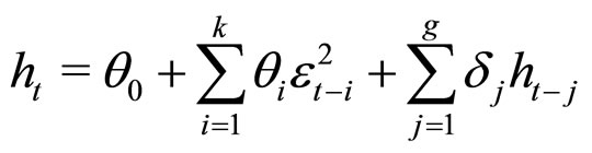 (5)
(5)
where,  are lagged unconditional variances and
 (6)
(6)
to ensure, positive variances exist. Realistically, GARCH(k,g) is an infinite order ARCH process with a rational lag structure imposed on the coefficients. The basic assumption in testing for ARCH effect is that linear serial dependence inside the original series is removed with a well fitted pre-whitening model and too, that any remaining serial dependence must be due to some nonlinear generating mechanism, which is not captured by the model. In this regard, the feature of interest here is the conditional heteroscedasticity, and that it is possible to show that the nonlinear mechanism remaining in the pre-whitened streamflow series, namely, the residual series, can be well interpreted as autoregressive conditional heteroscedasticity [1].
Thus to test for the ARCH effect, linear stochastic models: Deseasonalised ARMA(20,1) and AR(11) were developed for both the daily and monthly streamflow processes, respectively. Before model fitting, both streamflow processes were logarithmically transformed and deseasonalised based on classical harmonic analysis [6]. Before applying ARCH tests to the residual series, to ensure that the null hypothesis of no ARCH effect is not rejected due to the failure of the pre-whitening linear stochastic models, it is important to check the goodness-of-fit of the models. Figures 4 and 5 clearly show that the linear stochastic models fit the respective streamflow regimes appropriately, as there are no significant serial correlations present in the residual.
Despite this though, while the residuals seemed statistically uncorrelated according to the autocorrelation function (ACF) values (i.e., Figures 4 and 5), Figure 6 shows that the autocorrelation values are not identically distributed; that is, the residuals are not independent and identically distributed over time. This situation, basically, connotes volatility, a common behaviour of GARCH process.
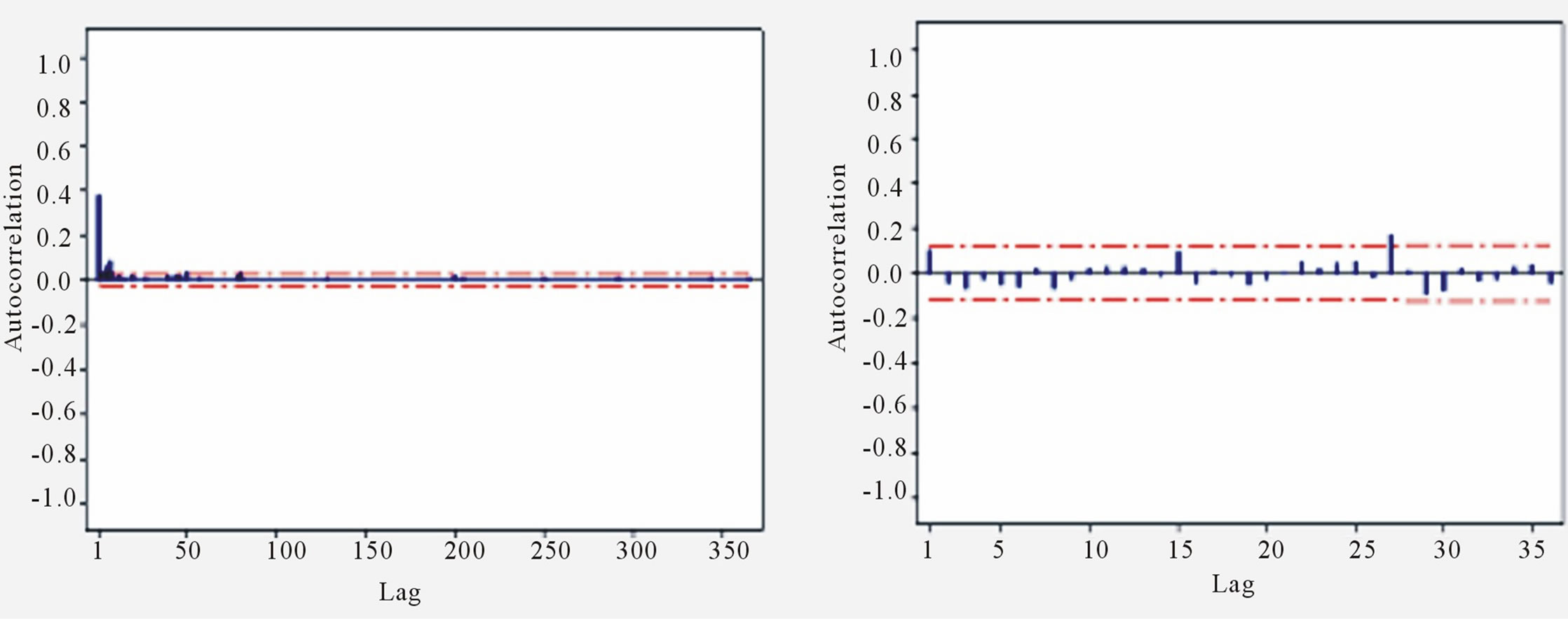
It has been noted that some of the series modelled by linear stochastic models exhibit autocorrelated squared residuals [7]. Figure 7 attests to this assertion.
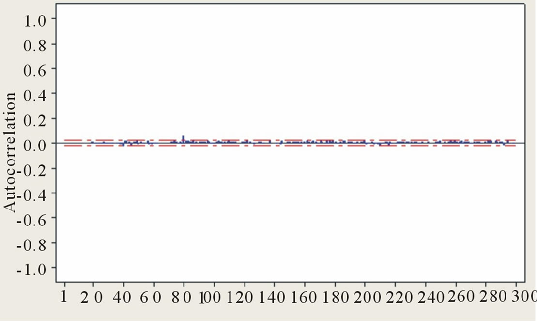
Figure 4. ACF of residuals from ARMA(20,1) model for daily flow.
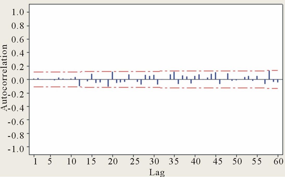
Figure 5. ACF of residuals from AR(11) model for monthly flow.
 (a) (b)
Figure 6. Segments of the residual series from (a) ARMA(20,1) for daily flow; (b) AR(11) formonthly flow.
 (a) (b)
Figure 7. Autocorrelation functions of the squared residuals from (a) ARMA(20,1) model fordaily flows and (b) AR(11) model for monthly flows.
Though, the residuals seemed almost uncorrelated over time, the squared residuals are clearly correlated (Figure 7). The autocorrelation structures of both squared residual series still exhibit traces of strong seasonality. The physical implication of this is that the variance of residual series is conditional on its past history; that is, the residual series may probably exhibit ARCH effect.
Thus to test for the presence or otherwise of ARCH effect, the Engle’s Lagrange Multiplier (LM) test and Ljung-Box-Pierce Q-test for a departure from randomness based on autocorrelation function of the data series were adopted and implemented using MATLAB routines. The test statistic for LM test is given by TR2, where R is the sample multiple correlation coefficients computed from the regression of  on a constant, and
  T is the sample size. Under the null hypothesis that there is no ARCH effect, the test statistic is asymptotically distributed as Chi-square distribution with q degrees of freedom. On the other hand, Ljung-BoxPirece test is a modification of the Box-Pierce test. The Ljung-Box-Pirece test for ARCH effect takes a look at the autocorrelation function of the squares of the prewhitened data, and tests whether the first L autocorrelations for the squared residuals are collectively small in magnitude. For fixed, sufficiently large L, the Ljung-BoxPierce Q-statistic is defined according as
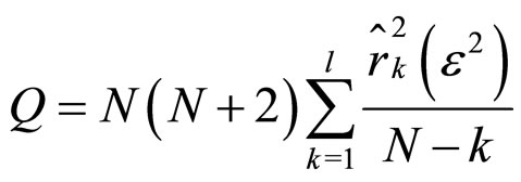 (7)
(7)
where, N is the sample size, and  is the squared sample autocorrelation of squared residual series at lag k. Like the Engle’s LM test, under the null hypothesis of a linear generating mechanism for the data, namely, no ARCH effect, the test statistic is asymptotically
  distributed.
2.3. Modelling Framework and Development
Attempts have been made by several researchers [1,8-10] to model both economic series and hydroclimatic processes by combining ARMA models with ARCH errors. The same framework was adopted in this study; here, the daily streamflow process was modelled by using ARMAGARCH regime. In this regard, the ARMA-GARCH model employed can be interpreted as a direct combination of an ARMA model which was used to model the mean behaviour and the ARCH, for ARCH effect in the residual series from the model. The general GARCH (p,q) model for the conditional variance of innovations is:
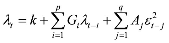 (8)
(8)
with constraints:
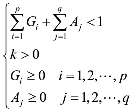 (9)
(9)
where,  denotes a real-valued discrete time stochastic process, p and q represent the order of the GARCH(p,q) conditional variance model; k is a constant, GARCH: represents the p-element coefficient vector Gi, and ARCH: represents the q-element coefficient vector Aj.
Since there is obvious presence of seasonality in the residuals of the daily streamflow under discourse, to preserve the seasonality in the variance of the residuals, the ARCH model was fitted to deseasonalised residual series. As a result, the ARMA-GARCH model with seasonal deviations was adopted. This model takes the form:
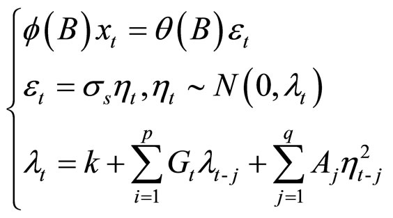 (10)
(10)
where,  is the seasonal standard deviation of
  and s is the season number depending on which season the time t, belongs to; for daily flow series, s ranges from 1 to 366. GARCH models can be treated as ARMA models for squared residuals; thus, its order was determined based on the method for selecting the order of ARMA models; the traditional model selection criteria such as Akaike information criterion (AIC) and Bayesian information criterion (BIC) were used for selecting the models.
According to the AIC, ACF and PACF structures, two GARCH models were found suitable; GARCH(0,7), i.e., ARCH(7) and GARCH(2,1) models. These models were selected based on the smallest AIC value for each of the cases considered. Hence, the preliminary ARMA-GARCH models fitted to the daily streamflow is composed of ARMA(20,1)-ARCH(7), and ARMA(20,1)-GARCH(2,1). On the basis of model parameter parsimony and significance, the latter was preferred. The model building process was done using the GARCH Tool Box in MATLAB. The parameter and AIC values for these models obtained during model fitting process were as follows, i.e., 1) and Table 1 in 2) below.
1) ARMA(20,1)-ARCH(7) Model PARAMETERS: c = 0.027344; k = 0.77497; ARCH(1): 0.32992; ARCH(2): 0.14675; ARCH(3): 0.000; ARCH (4): 0.018271; ARCH(5): 0.046449; ARCH(6): 0.00895; ARCH(7): 0.03078; AIC: 27718.76; BIC: 27783.17 2) ARMA(20,1)-GARCH(2,1) Model AIC: 27897.55; BIC: 27933.33
3. Results and Discussion
3.1. ARCH Effect
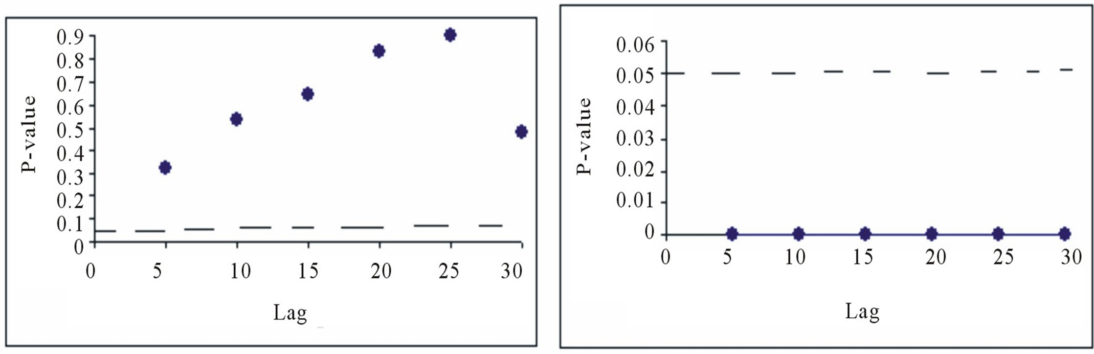
Tables 2 and 3 and Figure 8, show the Engle’s LM test for the residuals from both ARMA(20,1) and AR(11) for daily and monthly flow series.
As reported in Tables 2 and 3, H = 0 and H = 1, both respectively indicate that when the H = 0, it implies that no significant correlation exists in the series and by extension, no ARCH effect, especially with the pvalues greater than zero; similarly, H = 1 means there is presence of significant correlation and by implication, existence of the ARCH effect. From the results as shown in Tables 2 and 3, and Figure 8, the Engle’s LM test for the residuals indicate the existence of ARCH effect in the AR-MA (20,1) model for daily flow, whereas the null hypothesis of no ARCH effect is accepted for the residuals of the AR (11) model for monthly flow; Figure 8(a) clearly illustrates that there is no significant autocorrelation left in the monthly flow residuals.
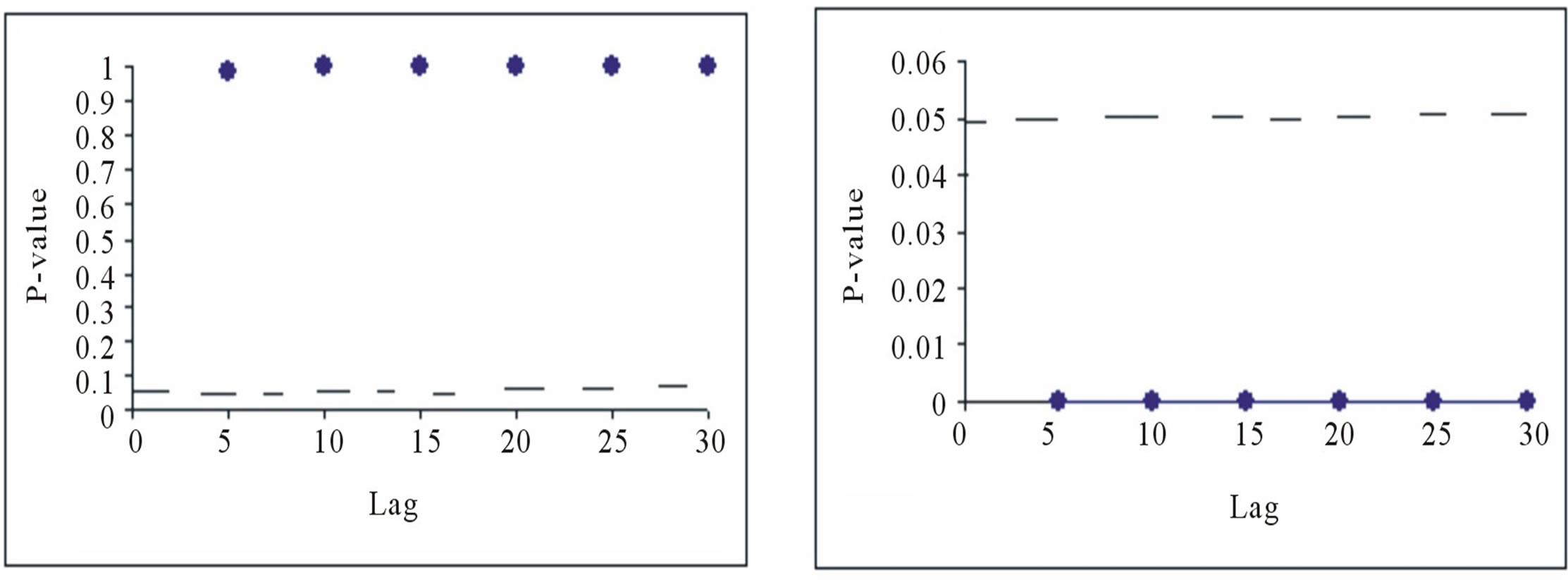
Figure 9 and Tables 4 and 5 report the results of the Ljung-Box-Pierce test for ARCH effect. Based on the Ljung-Box test, the null hypothesis of no ARCH effect is rejected for the residuals from ARMA(20,1) of the daily flow, whereas the result is to the contrary for the residuals from AR(11) of the monthly flow series; this result confirms that there is no significant autocorrelation left in the monthly flow residuals.
On the whole, based on the test statistics in the two cases, it is clear that there is existence of conditional heteroscedasticity in the residual series from linear model (ARMA(20,1)) fitted to deseasonalised logarithmic-transformed daily streamflow process; but for monthly flow, the deseasonalisation pre-processing has successfully removed the seasonal variance in the monthly flow series, as indicated by both the Engle’s LM and Ljung-Box tests for ARCH effect on the residuals of the AR(11) fitted to it. From the results, it is important to note that the higher the time frequency, the greater both the test statistics (i.e., Ljung-Box and Engle’s LM) exceeds the critical value.
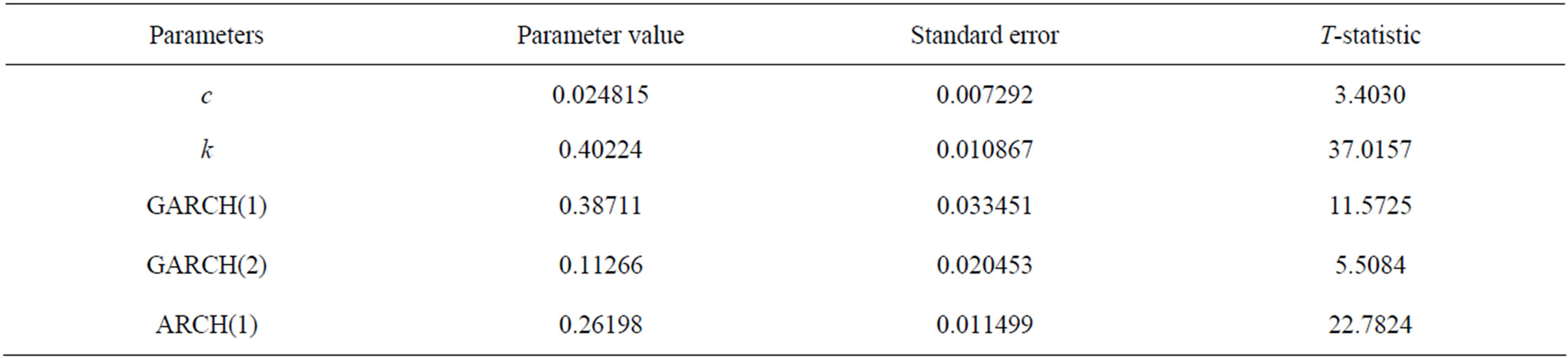
Table 1. ARMA(20,1)-GARCH(2,1) model fitting.

Table 2. Engle’s LM test (Daily flow).
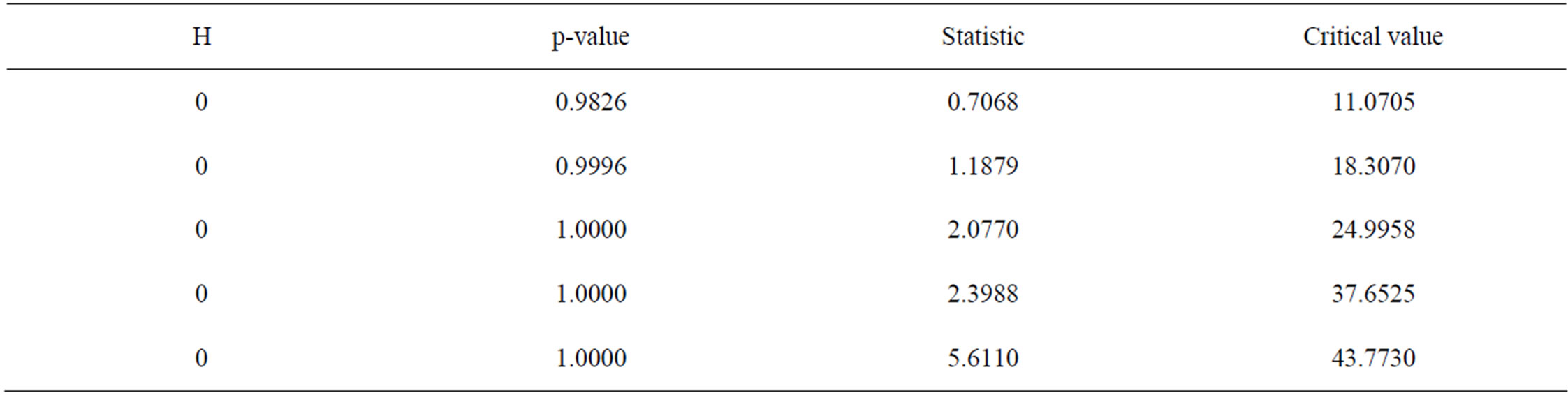
Table 3. Engle’s LM test (Monthly flow).
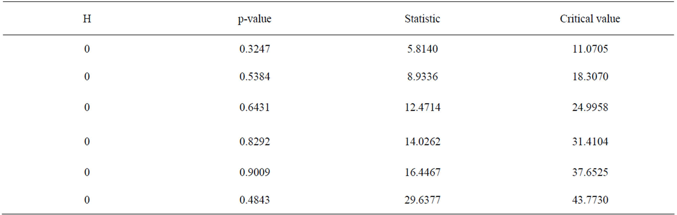
Table 4. Ljung-box-pierce test (Monthly flow).
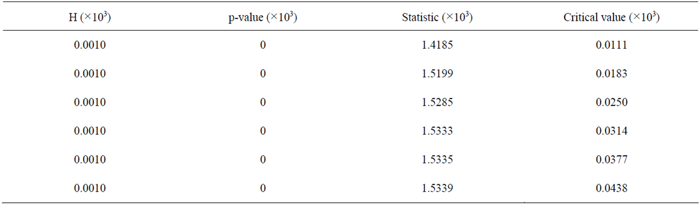
Table 5. Ljung-box-pierce test (Daily flow).
 (a) (b)
Figure 8. Engle’s LM test for residuals from (a) AR(11) model for monthly flow and (b) ARMA(20,1) model for daily flow.
 (a) (b)
Figure 9. Ljung-Box Q-test for the residuals from (a) AR(11) model for monthly flow and (b) ARMA(20,1) model for daily flow.
3.2. Model Development
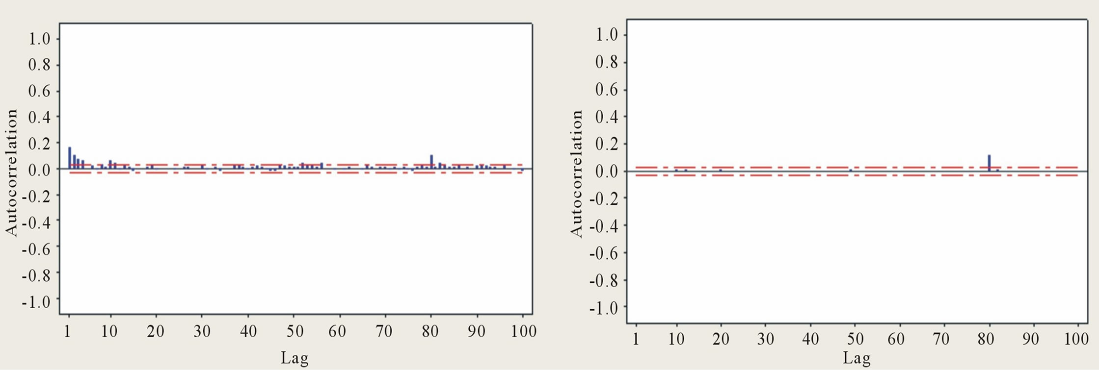
If the ARMA-GARCH model is successful in modelling the serial correlation in the conditional mean and conditional variance, there should be no autocorrelation left in both the residuals and the squared residuals standardised by the estimated conditional standard deviation. Figure 10 shows segments of the seasonally standardised residual series from the ARMA(20,1) model and its corresponding conditional standard deviation sequence estimated with GARCH(2,1) model. The standardisation of the residual series from the ARMA(20,1) model was effected by dividing by the estimated conditional standard deviation sequence. The autocorrelations of the standardised residuals and the corresponding squared standardised residuals are as plotted in Figure 11. Figure 11 shows that even though there is no autocorrelation in the squared residuals (Figure 11(b)), which implies that the ARCH effect has been removed, but in the nonsquared standardised residuals (Figure 11(a)), there is still presence of weak autocorrelation. Tables 6-10 and Figure 12 show the test results for ARCH effect on the standardised residuals from both ARMA(20,1)-GARCH (0,7) and ARMA(20,1)-GARCH(2,1) models; the test results indicate very clearly that the ARCH effect has been removed.
Because the GARCH is designed to deal with the conditional variance behaviour, rather than mean behaviour, the weak autocorrelation still present in the non-squared residual series must have arisen from the seasonally standardised residuals of the ARMA-GARCH building process. However, since tests for ARCH effect revealed that the model passed the test; i.e., the null hypothesis of no ARCH effect is accepted, there is no further need at this juncture to re-fit the data. Despite this though, it should be noted that a wrongly-specified ARMA model may lead to unclear structure in the autocorrelations and partial autocorrelations of the residual series; a wrongly-specified ARMA model has little explanatory
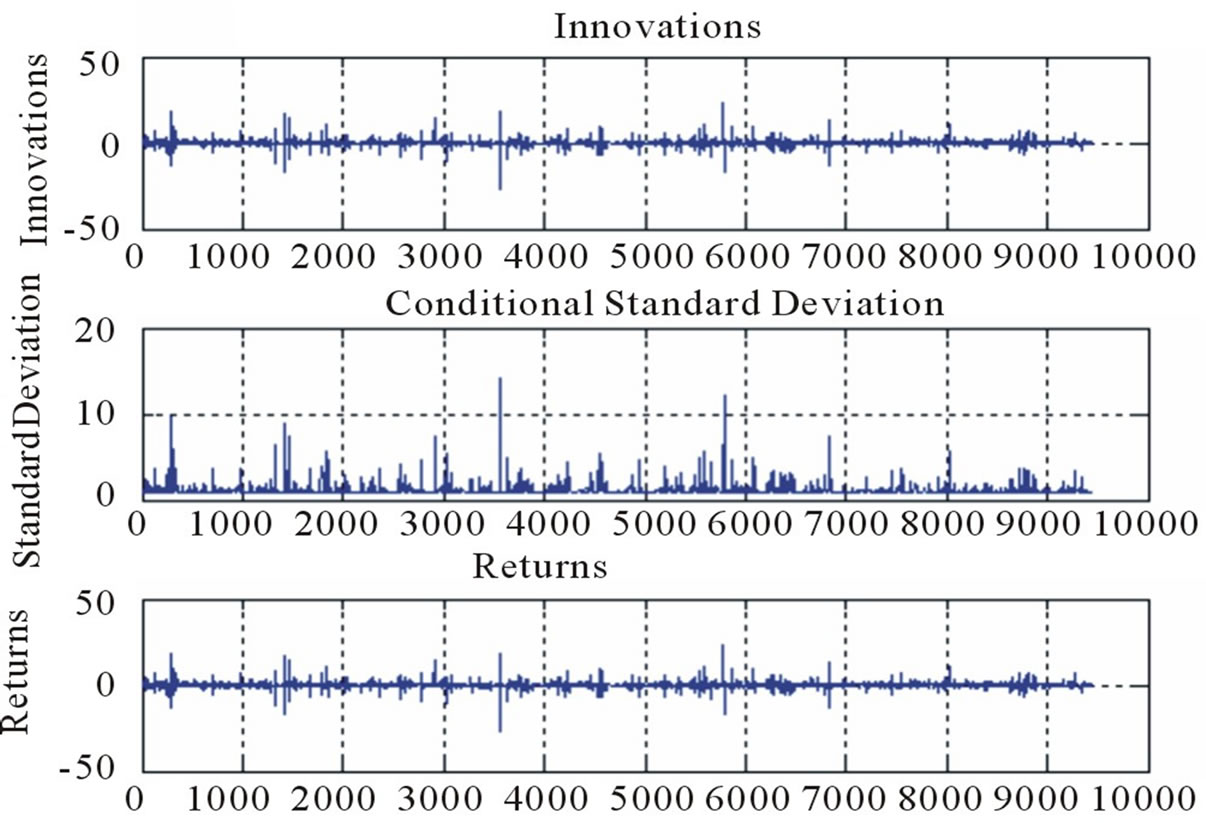
Figure 10. GARCH(2,1) model fitted to the seasonally standardised residuals from ARMA(20,1) model for daily flow; Note: (a) Returns as used here represent the observed residuals, i.e., seasonally standardised residuals; (b) Innovations stand for the residuals from the GARCH(2,1) model fitted to the observed residuals.
 (a) (b)
Figure 11. Autocorrelation functions of (a) standardised residuals, and (b) squared standardised residuals from ARMA(20,1)- GARCH(2,1) model.
 (a) (b)
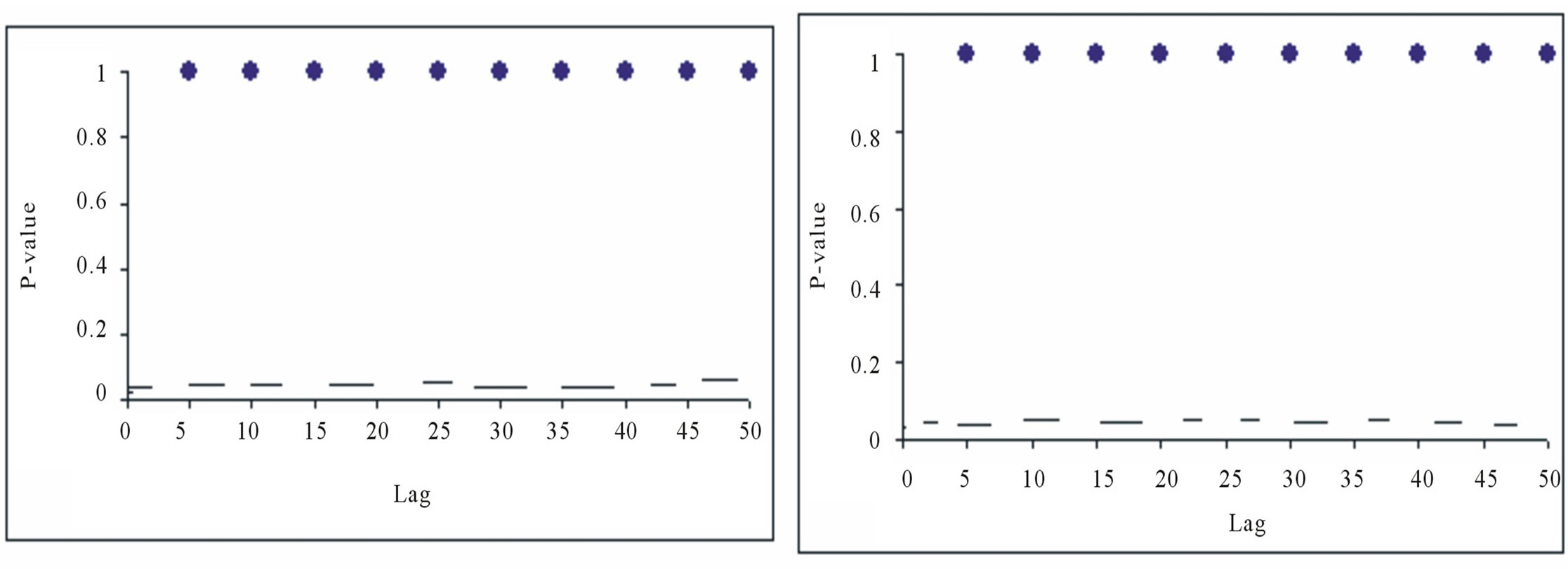
Figure 12. Tests for ARCH effect: (a) Ljung-Box test and (b) Engle’s LM test for standardised residuals from ARMA(20,1)- GARCH(2,1) model for daily flow.
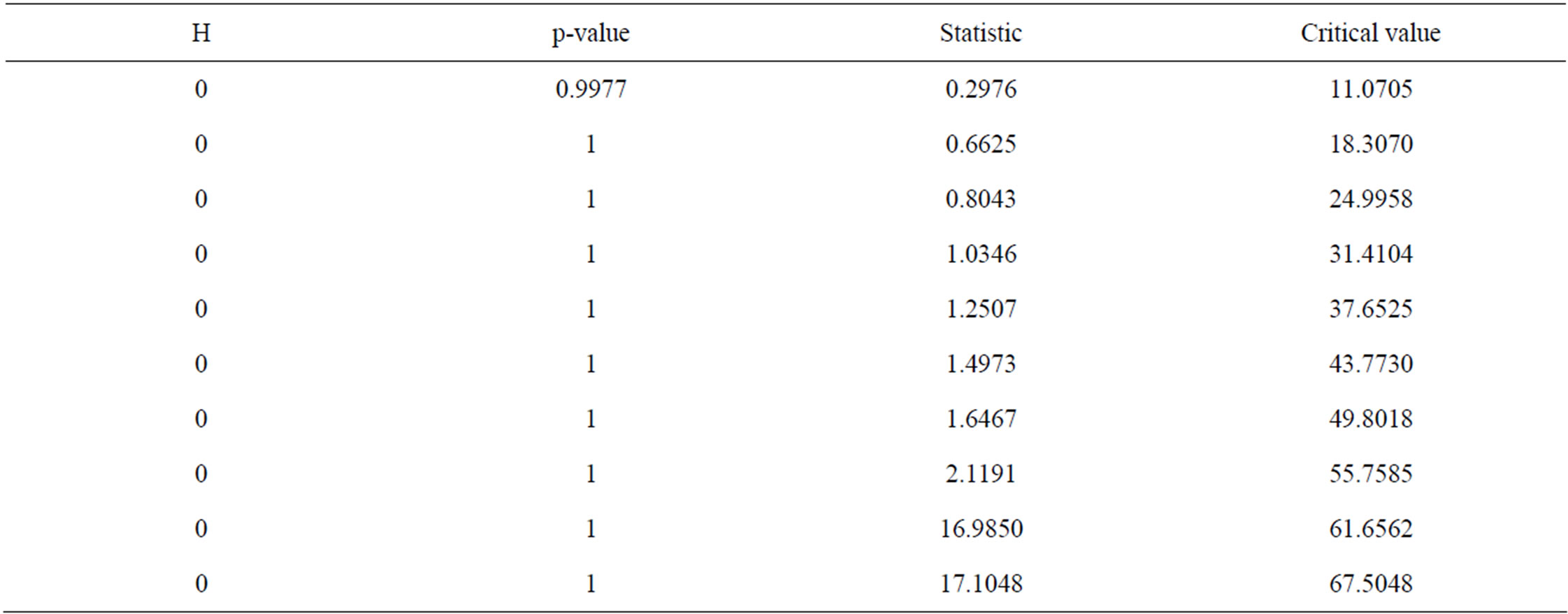
Table 6. Engle’s LM test on standardised residuals from ARMA(20,1)-ARCH(7) model.
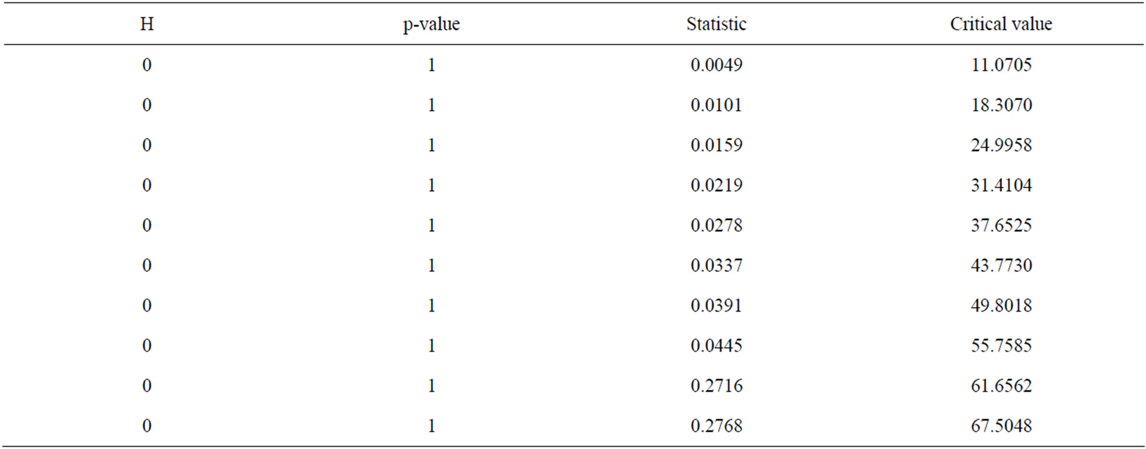
Table 7. Engle’s LM test on squared standardised residuals from ARMA(20,1)-ARCH(7).
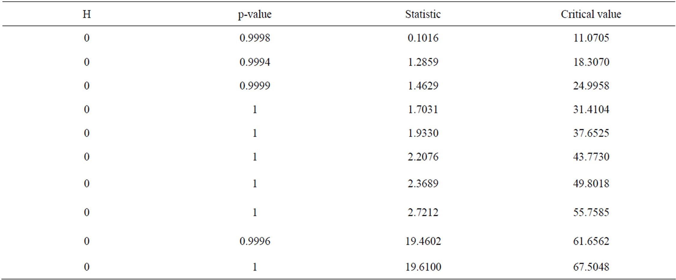
Table 8. Ljung-Box test on squared standardised residuals from ARMA(20,1)-GARCH(2,1).
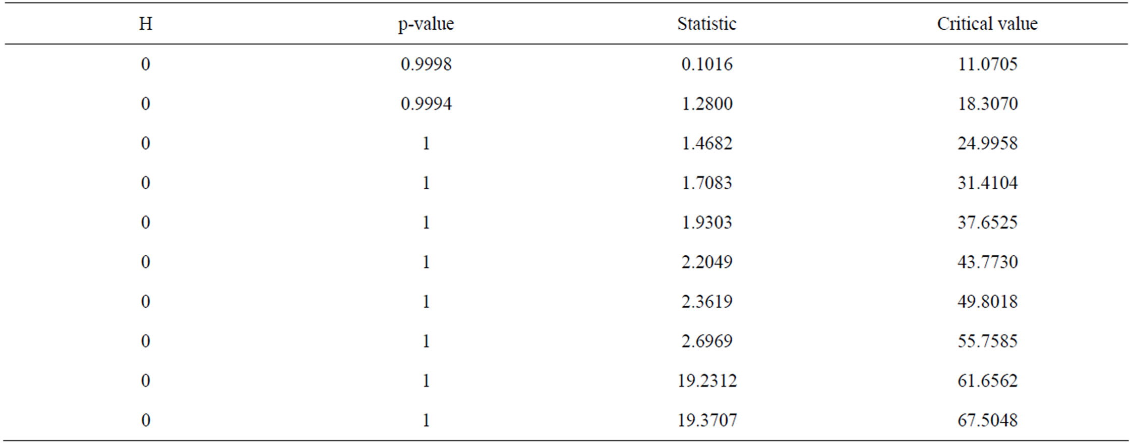
Table 9. Engle’s LM test on standardised residuals from ARMA(20,1)-GARCH(2,1).
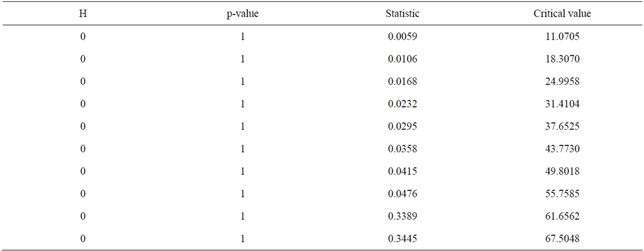
Table 10. Engle’s LM test on squared standardised residuals from ARMA(20,1)-GARCH(2,1).
power in all instances. In addition, a GARCH model may be better disposed to capture observed nonlinear dynamics, and a tendency to reduce serial dependence and leptokurtosis, it could become inadequate to model the generating mechanism in the flow process if the autocorrelations of the squared residual process of the series decay so slowly. As reported in Bera and Higgins [11], the third moment for a regular ARCH process is zero; therefore, unconditional distributions of the series must be symmetric. Though, the conventional ARCH or GARCH model is able to capture the excessive kurtosis, as usually the case in most hydrological time series, it cannot capture asymmetry.
3.3. Pre-Whitening Linear Stochastic Models
Linear stochastic models like SARIMA, deseasonalised ARMA, and periodic models are the most commonly used in modelling hydrological processes. Considering model formulation in terms of the constitutive equation, though the seasonal variation in the variance present in the original time series can be dealt with basically by the deseasonalisation approach, neither of the SARIMA and ARMA models take into account the seasonal variation in variance of the residual series; it is primarily due to the fact that the innovation series is assumed to be independent and identically distributed. Hence, both SARIMA and deseasonalised models cannot capture the ARCH effect usually observed in the residual series [1].
In contrast, the periodic model, which is another version of ARMA models, which is fitted to separate seasons, allows for seasonal variances in not only the original series but also the residual series. Periodic models have a high potential to perform better than both SARIMA and deseasonalised ARMA models in capturing the ARCH effect since it takes into account season-varying variances [1]. But however, while seasonal variances might be sufficient for describing ARCH effect in monthly flow series, because in monthly flows, it is caused by seasonal variances, the contrary is the case with daily flow series.
4. Conclusions
It is obvious from available literature that discussions on the nonlinear mechanism, conditional heteroscedasticity in hydrological processes have been very austere. Modelling data with time varying conditional variance could be attempted in various ways, non-parametric and parametric. Towards this end, the parametric approach was adopted here. The existence of the ARCH effect was verified in the residual series from linear models fitted to the monthly and daily streamflow processes. Following from the tests, it is shown that the ARCH effect is caused by seasonal variation in the variance for monthly flows, but seasonal variation in variance can only partly explain the ARCH effect in daily streamflow. It is also evident that the traditional seasonal ARMA models are inadequate in describing ARCH effect in the daily streamflow process; though, PARMA model is adequately robust in describing monthly flows by considering season-dependent variances. In the light of this, and taking the seasonal variances inspected in the residuals from linear stochastic models fitted to the daily flow series into consideration, the idea of an ARMA-GARCH model with seasonal components is worth exploring.
The ARMA-GARCH model is basically a combination of an ARMA model, which is used to model the mean behaviour, and GARCH model, the ARCH effect in the residuals from the ARMA model. Thus, to preserve the seasonal variation in variance in the residuals, the ARCH model should not be fitted directly to the residual series, but rather, to seasonally standardized residuals. Because the ARCH effect in daily streamflow could mainly arise from perturbations in daily hydroclimatic variations, the spread in the use that may accrue from developing an ARMA-GARCH model could be limited. Despite this though, because the relationship regime between runoff and rainfall on one hand, and rainfall and temperature on the other is complex to capture precisely by any model, and too, the non-availability of large enough rainfall data, the accuracy of weather forecasts could be limited. Thus, the potential of an ARMA-GARCH model should be explored and probably embraced for modelling daily streamflow, at least in terms of the relevance of statistical modelling in hydrology.
REFERENCES
- W. Wang, P. H. A. J. M. Van Gelder, J. K. Verjling and J. Ma, “Testing and Modelling. Autoregressive Conditional Heteroscedasticity of Streamflow Processes,” Nonlinear Processes in Geophysics, Vol. 12, 2005, pp. 55-66. doi:10.5194/npg-12-55-2005
- V. Livina, Y. Ashkenazy, Z. Kizner, V. Strygin, A. Bunde and S. Havlin, “A Stochastic Model of River Discharge Fluctuations,” Physica A, Vol. 330, No. 1-2, 2003, pp. 283-290. doi:10.1016/j.physa.2003.08.012
- M. Y. Otache, “Contemporary Analysis of Benue River Flow Dynamics and Modelling,” Ph.D. Dissertation, Hohai University, Nanjing, 2008.
- M. Y. Otache, A. S. Mohammed and I. E. Ahaneku, “NonLinear Deterministic Chaos in Benue River Flow Daily Time Series,” Journal of Water Resource and Protection, Vol. 3, No. 10, 2011, pp. 747-757.
- T. Bollerslev, “Generalized Autoregressive Conditional Heteroscedasticity,” Journal of Econometrics, Vol. 31, No. 3, 1986, pp. 307-327. doi:10.1016/0304-4076(86)90063-1
- N. T. Kottegoda, “Stochastic Water Resources Technology,” The Macmillan Press Ltd., London, 1980.
- C. W. J. Granger and A. P. Andersen, “An Introduction to Bilinear Time Series Models,” Vandenhoeck and Ruprecht, Gottingen, 1978.
- A. A. Weiss, “ARMA Models with ARCH Errors,” Journal of Time Series Analysis, Vol. 5, No. 2, 1984, pp. 129-143. doi:10.1111/j.1467-9892.1984.tb00382.x
- M. A. Hauser and R. M. Kunst, “Fractionally Integrated Models with ARCH Errors: With an Application to the Swiss 1-Month Euromarket Interest Rate,” Review of Quantitative Finance and Accounting, Vol. 10, No. 1, 1998, pp. 95-113. doi:10.1023/A:1008252331292
- R. J. S. Tol, “Autoregressive Conditional Heteroscedasticity in Daily Temperature Measurements,” Environmetrics, Vol. 7, No. 1, 1996, pp. 67-75. doi:10.1002/(SICI)1099-095X(199601)7:1<67::AID-ENV164>3.0.CO;2-D
- A. Bera and M. Higgins, “On ARCH Models: Properties, Estimation, and Testing,” In: L. Oxley, D. A. R. George, C. J. Roberts and S. Sayer, Eds., Surveys in Econometrics, Blackwell Press, Oxford, Cambridge, 1995, pp. 171-224.