Open Journal of Modern Hydrology
Vol. 2 No. 2 (2012) , Article ID: 18560 , 8 pages DOI:10.4236/ojmh.2012.22006
SWAT and Wavelet Analysis for Understanding the Climate Change Impact on Hydrologic Response
![]()
1Institute for a Secure and Sustainable Environment, University of Tennessee, Knoxville, USA; 2Bechtel Corporation, Houston, USA.
Email: skoirala@utk.edu
Received January 17th, 2012; revised February 1st, 2012; accepted February 21st, 2012
Keywords: Climate Change; SWAT; Wavelet; Hydrologic Response
ABSTRACT
Quantifying the hydrological response to an increased atmospheric carbon dioxide concentration and climate change is important in a watershed scale particularly from the application point of view. The specific objectives are to evaluate the climate change impact on the future water yield at the outlet of Clinch River Watershed upstream of Norris Lake in Tennessee, USA and see how the frequency of extreme water yield (e.g. flood) changes compared to present condition. The predicted future climate change by climate change scenarios A2 from community climate system model (CCSM) is applied. The model was calibrated using monthly average streamflow data from 1970 to 1989 and validated using similar data from 1990 to 2009 collected at a USGS gauging station 03528000. Changes in monthly average streamflow were estimated for long term (around 2099). Results were also interpreted in the time-frequency domain approach by showing how frequency of occurrence changes based on A2 scenario.
1. Introduction
Climate change will likely affect fundamental drivers of the hydrological cycle and has a wide range of consequences for human societies and ecosystems. According to Intergovernmental Panel on Climate Change (IPCC) fourth assessment report (AR4), observed global warming has been linked to changes in the large-scale hydrological cycles such as: changes in precipitation patterns, intensities, extremes, and changes in soil moisture and runoff. However, our ability to interpret changes in impact-relevant variables (e.g. changes in circulation, precipitation and extremes) remains limited [1]. More understanding of the processes driving the changes at different temporal and spatial scales could be beneficial. So IPCC AR4 recommended more research to improve the ability of models related to circulation and precipitation patterns, extremes, El-Nino and seasonal variability, hydrological cycle both in a short and long terms. It also recommended to increase the focus on regional and watershed scale climate study. Improved understanding of how climate change could influence the hydrological cycle and water resources in a regional and watershed scale is identified as a major research priority.
Since there is a regional variation of hydrologic conditions, the influence of climate change on hydrology in watershed scale may also vary between watersheds even under the same climate scenarios. Many recent studies indicate the importance of watershed scale climate variability due to global climate change particularly for long-term water resources planning and management [2, 3].
The hydrologic models should provide a link between climate changes and water yields through simulation of hydrologic processes within watersheds. However, most hydrologic models are unable to incorporate the climate change effect for simulation. The Soil and Water Assessment Tool (SWAT) [4] is one widely used model which has the capability of incorporating the climate change effect for simulation. In SWAT, it is possible to incorporate the general circulation model (GCM) projections of carbon dioxide concentration, precipitation and temperature changes. Hence SWAT was used in this study.
Most of the research related to the impact of climate change on water resources is focused on comparing the water yield in future, based on different climate change scenarios [5,6]. However, there is a limited research on how the frequency of occurrence of water yield changes compared to the present condition which in fact is particularly important from long term water resources planning and management point of view. In this study we attempt to explore this issue. The specific objectives are to evaluate the climate change impact on the future water yield at the outlet of Clinch River Watershed upstream of Norris Lake in Tennessee and see how the frequency of extreme water yield (e.g. flood) changes compared to present condition.
The Intergovernmental Panel on Climate Change (IPCC) published a set of emission scenarios in the Special Report to serve as a basis for assessments of future climate change [1,2]. Among different scenarios, the A2 scenario was chosen for this study because it represents a plausible condition over the next century and this is one of the most widely simulated over all models [7]. The A2 scenario is characterized by a world of independently operating, self-reliant nations, continuously increasing population, regionally oriented economic development, and slow and more fragmented technological changes and improvements to per capita income [1]. It should be noted that not all modeling groups have runs for all emission scenarios.
The outline of the paper is as follows. Section 2 describes the research site and data used in the analysis. Section 3 presents the methodology with detailed description on statistical analysis and wavelet transform. Results are presented and discussed in Section 4 and Section 5 concludes the paper.
2. Site and Data Description
The Clinch River is one of the tributaries of the Tennessee River. The Clinch River watershed in Tennessee, was selected for study because this watershed in the Tennessee River Basin was one of the basins which has not regulated and this may represent the natural watershed response. The watershed is a 3,818 square kilometer forested watershed (Figure 1).
Climate data required by the model are daily precipitation, minimum and maximum daily air temperature, solar radiation, wind speed and relative humidity. These daily climatic inputs can be entered from historical records, and/ or generated internally in the model using monthly climate statistics that are based on long-term weather records and are available internally in the SWAT database for US. In this study, daily total rainfall, daily maximum and minimum temperature are obtained from four weather stations within and near the watershed from 1970 to 2009. Monthly average discharge for calibration and validation was also used from 1970 to 2009 from USGS gauge station 03528000 at the outlet of the water-

Figure 1. Study area location map.
shed upstream of the Norris Lake (Figure 2). Rest of the climate data required were generated internally in SWAT.
Elevation data were obtained from USGS 30 m Digital Elevation Models (DEMs). Elevation ranges from 321 m to 1429 m from mean sea level (Figure 2). Landuse data were obtained from 1:24,000 NLCD database. Soil data were obtained from the State Soil Geographic (STASTGO) database.
3. Methodology
Before Delineation of watershed, subwatersheds and creation of stream networks were based on a USGS digital elevation model (DEM) with 30 m grid cell resolution by specifying the threshold drainage area and the watershed outlet. The threshold area is the minimum drainage area required to form the origin of the stream [6] . The watershed outlet was selected at the USGS gage station to compare the simulated and observed data. The threshold area of 8,000 ha created 19 subwatersheds as shown in Figure 2. Each of these subwatershed is further divided into Hydrological Response Units (HRUs) based on the defined threshold of landuse, soil and elevation characteristics. The defined threshold for landuse, soils and elevation were 10%, 10% and 5% respectively, which created 297 HRUs.
3.1. Statistical Analysis
The Coefficient of determination (R2) is an indicator of the strength of the relationship between the observed and simulated values which ranges from 0 to 1. The Nash-Sutcliffe efficiency (E) indicates how the plot of the observed and simulated values fit the 1:1 line, which ranges from negative infinity to 1. The formula to calculate R2 and E are given by [2,8,9],
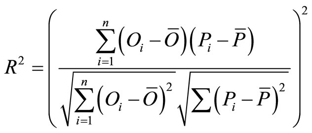 (1)
(1)
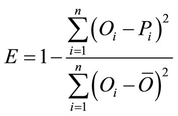 (2)
(2)
where O represents the observed value and P represents the predicted value. The over bar is the mean for the entire time period of evaluation, and i = 1, 2, 3···n, where n is the total number pairs of data.
3.2. Wavelet Analysis
The wavelet transform is a method of converting a
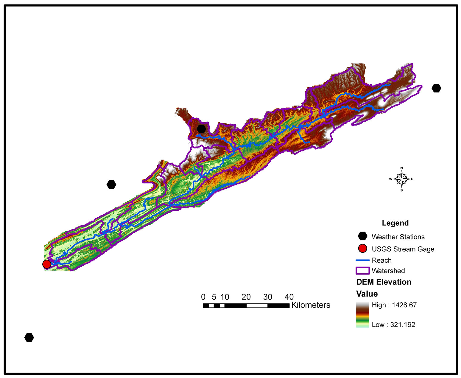
Figure 2. Digital elevation model of the study area.
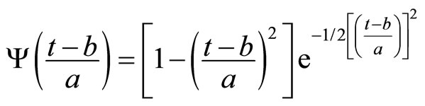
function (or signal) into another form which either makes certain features of the original signal more amenable to study or enables the original data set to be described more succinctly [10]. In the wavelet transform, an energy spectrum describes in the frequency domain what the autocorrelation function expresses in the time domain. The amplitude of the spectrum, however, allows visualization of the frequency content of the time series and is more useful for comparing signals to each other and for isolating meaningful frequency peaks [11]. To perform the transform, a wavelet, which is a localized waveform and function that satisfies certain mathematical criteria, is needed. A Mexican-hat wavelet was chosen for the analysis because of our focus on the amplitude of the wavelet spectrum [12]. The Mexican-hat wavelet for time t is defined as:
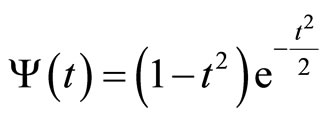 (3)
(3)
which is the second derivative of the Gaussian distribution function .
.
Equation (3), is defined as the mother wavelet or analyzing wavelet. This is the basic form of the wavelet from which dilated and translated versions are derived and used in the wavelet transform as presented in Equation (4) The dilation and contraction are governed by the dilation parameter a, which is the distance between the center of the wavelet and its intersection with the time axis. The movement of the wavelet along the time axis is governed by the translation parameter b. The translated and dilated form of the altered mother wavelet is defined in equation (4).
 (4)
(4)
From equation (4), a transformed signal,  , can be defined using a range of a’s and b’s. The wavelet transform of a signal
  is thus defined as
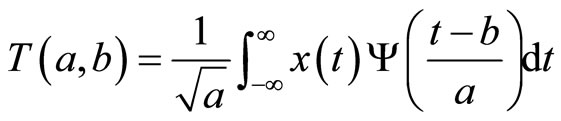 (5)
(5)
The wavelet spectral power is estimated from this convolution integral using the following expression:
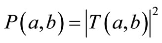 (6)
(6)
A plot of the spectral power is obtained by varying a and b and is plotted against the time scale.
A MATLAB code developed by Torrence and Compo [12] was used for the analysis.
First the Coefficient of Determination (R2) and The Nash-Sutcliffe efficiency (E) are determined from the calibrated and validated model input/output using the Equations (1) and (2). Monthly water yield and the projected monthly water yield time series from the model output are processed using the MATLB code for wavelet transform, which primarily uses the Equations (3)-(6).
4. Results and Discussion
4.1. Sensitivity Analysis, Calibration and Validation
Potential evapotranspiration was modeled with the Penman-Monteith algorithm, while surface runoff was modeled with the Curve number and the variable storage channel routing approach. Initial model simulations were conducted using the default range of values for most model parameters using parameter solution (PARASOL) within SWAT-CUP. Table 1 shows the most sensitive parameters. Groundwater delay time (GW_DELAY), Manning’s N value for the channel (CH_N2), baseflow alpha factor for bank storage (ALPHA_BNK), soil evaporation compensation factor (ESCO), effective hydraulic conductivity (CH_K2), initial SCS curve number (CN2), baseflow alpha factor (ALPHA_BF) and maximum canopy storage (CANMX) are most sensitive values which are statistically significant within 95% confidence level as shown in Table 1. These significant values are adjusted to find the best parameter values for calibration.
Following the sensitivity analysis, SWAT monthly calibration was carried out using the data from January 1970 to December 1989. The results were then assessed based on the visual agreement observed and simulated streamflow plots and the performance statistics generated i.e. R2 and E which are 0.71 and 0.70 respectively (Figure 3).
Similar results were obtained for validation period which ranges from January 1990 through December 2009 with R2 estimate of 0.66 and E estimate of 0.65 as shown in Figure 4.
Although the model overestimated the higher discharge values and slightly underestimated the baseflow, it is generally a good agreement between the observed and the simulated data as indicated by R2 and E. The study area is in the karst zone which makes the simulation very complex. For comparison, in future we are also planning to perform more analysis using different approach such as wavelet analysis which may give better result in such complex karstic watershed.
4.2. Climate Change Scenario
For the A2 scenario test of climate change effects, the changes in temperature and precipitation were estimated using the CCSM downscaled data for the period of 2080 through 2099. Monthly changes in precipitation and temperature compared to present scenario are shown in
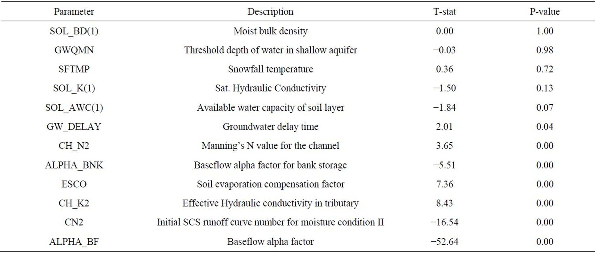
Table 1. Sensitivity analysis of parameters.
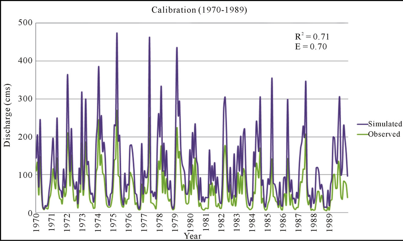
Figure 3. Calibration.
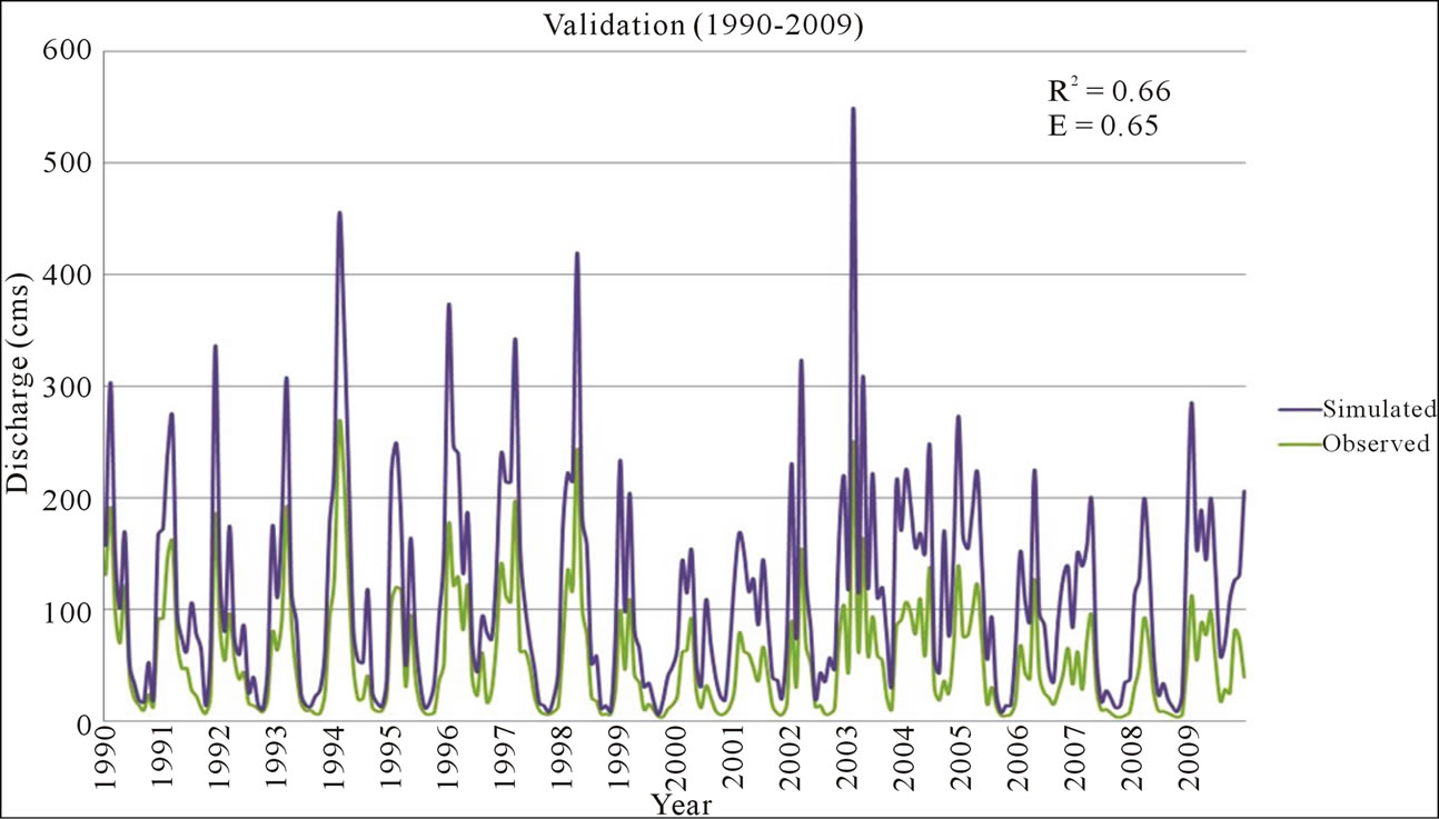
Figure 4. Validation.
Table 2. Summer and early fall (i.e. from May to September) months experience the highest increase in precipitation whereas there is a slight decrease in precipitation in December and January. There is always the increase in temperature ranging from 2.92 degree C in January to 5.22 degree C in June (Table 2). These changes were incorporated in the SWAT model and run the validated model to estimate the changes in water yield. Percentage change in average monthly water yield is shown in Figure 5. Increase in monthly water yield is highest in September, which is about 200% more than current condition. This may have tremendous effect on downstream flooding.
4.3. Wavelet Analysis
Our results showed that the significant peaks for precipitation occurred at 12, 36 and 85 months for the baseline period (1980 to 1999) (Figure 6). However for future climate condition (i.e. A2 scenario, from 2080 to 2099), there is one additional significant periodicity at around 18 months (Figure 7). Similarly, there was only one significant periodicity of water yield in the current base line period but in the future climate change scenario, there is one additional significant periodicity at 18 months. These results indicate that there is of course a change in frequency of occurrence of extreme events (e.g. flood) in addition to the increase in rainfall and discharge events.
5. Conclusions
In this study, some assessments were performed to evaluate the climate change impact on the future water yield at the outlet of Clinch River Watershed upstream of Norris Lake in Tennessee and see how the frequency of extreme water yield (e.g. flood) changes compared to present condition. SWAT hydrologic model was used to simulate the rainfall runoff relation. The model was calibrated and then validated using the USGS stream flow data at the watershed outlet. The validated model was used to predict the future water yield based on community climate system model (CCSM) downscaled rainfall and temperature data for A2 climate change scenario. The results clearly indicate the increase in flooding events as well as its frequency of occurrence in the future. Therefore, if the climate change scenario adopted for this
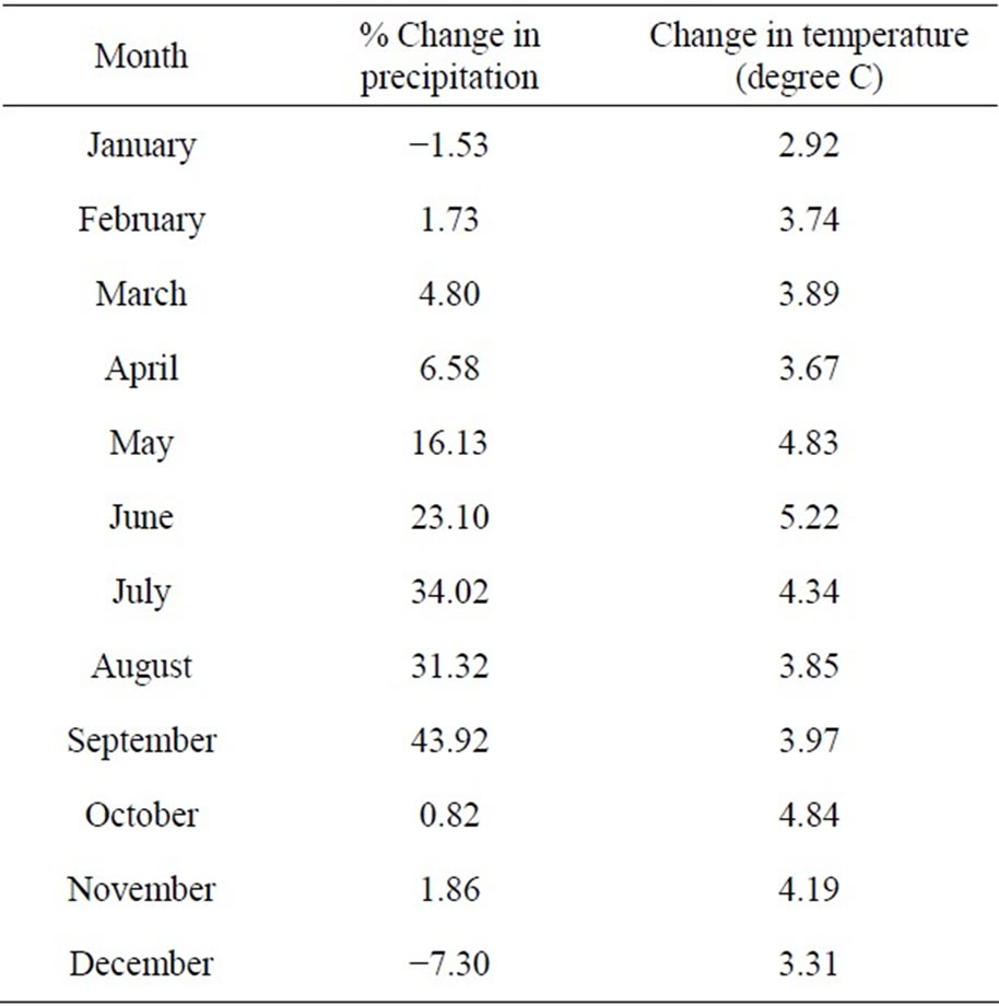
Table 2. Projected change in precipitation and temperature in 2099 based on CCSM A2 scenario compared to current condition (1980-1999).
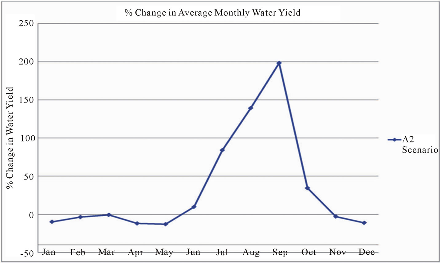
Figure 5. Percentage change in monthly water yield.

Figure 6. Monthly water yield (mm) from 1980 to 1999 (a) time series (b) corresponding wavelet spectrum (c) global wavelet spectrum.
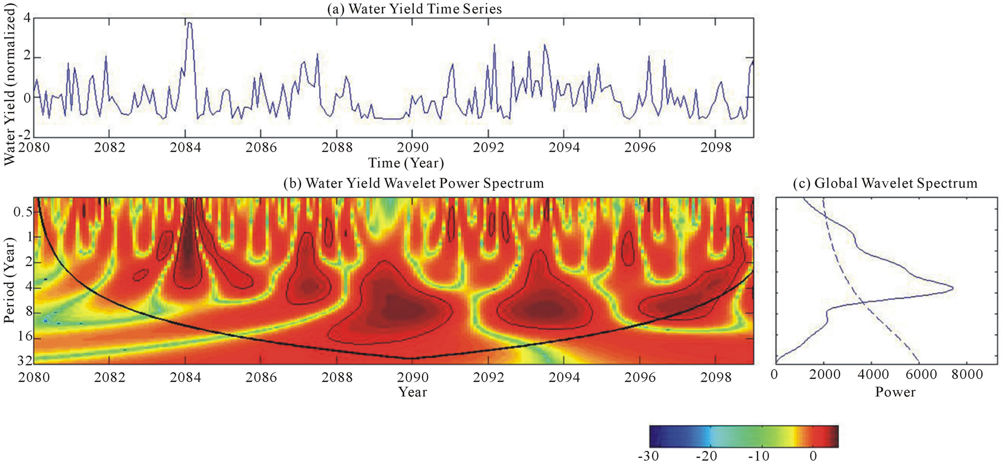
Figure 7. Projected monthly water yield (mm) from 2080 to 2099 based on A2 scenario (a) time series (b) corresponding wavelet spectrum (c) global wavelet spectrum.
study were to occur in the future, significant changes in the Tennessee and Cumberland Rivers could occur. There is a need to study implications of various mitigation strategies including the reviewing of downstream reservoir operation procedure to minimize the impact of climate change.
REFERENCES
- S. Solomon, “Intergovernmental Panel on Climate Change, and Intergovernmental Panel on Climate Change,” In: Working Group I, Climate change 2007: the physical science basis: contribution of Working Group I to the Fourth Assessment Report of the Intergovernmental Panel on Climate Change 2007, Cambridge, Cambridge University Press, New York, 996 p.
- X. Zhang, R. Srinivasan and F. Hao, “Predicting Hydrologic Response to Climate Change in the Luohe River Basin Using the SWAT Model,” Transactions of the ASABE, Vol. 50, No. 3, 2007, pp. 901-910.
- L. D. Brekke, et al., “Climate Change Impacts Uncertainty for Water Resources in the San Joaquin River Basin, California,” Journal of the American Water Resources Association, Vol. 40, No. 1, 2004, pp. 149-164. doi:10.1111/j.1752-1688.2004.tb01016.x
- J. G. Arnold, et al., “Large Area Hydrologic Modeling and Assessment Part 1: Model Development,” Journal of the American Water Resources Association, Vol. 34, No. 1, 1998, pp. 73-89. doi:10.1111/j.1752-1688.1998.tb05961.x
- D. L. Ficklin, et al., “Climate Change Sensitivity Assessment of a Highly Agricultural Watershed Using SWAT,” Journal of Hydrology, Vol. 374, No. 1-2, 2009, pp. 16-29. doi:10.1016/j.jhydrol.2009.05.016
- M. Jha, et al., “Climate Change Sensitivity Assessment on Upper Mississippi River Basin Streamflows Using SWAT,” Journal of the American Water Resources Association, Vol. 42, No. 4, 2006, pp. 997-1015. doi:10.1111/j.1752-1688.2006.tb04510.x
- N. S. Christensen and D. P. Lettenmaier, “A Multimodel Ensemble Approach to Assessment of Climate Change Impacts on the Hydrology and Water Resources of the Colorado River Basin,” Hydrology and Earth System Sciences, Vol. 11, No. 4, 2007, pp. 1417-1434. doi:10.5194/hess-11-1417-2007
- D. R. Maidment, “Handbook of Hydrology,” McGraw-Hill, New York, 1993.
- D. R. Legates and G. J. McCabe, “Evaluating the Use of ‘Goodness-of-Fit’ Measures in Hydrologic and Hydroclimatic Model Validation,” Water Resources Research, Vol. 35, No. 1, 1999, pp. 233-241. doi:10.1029/1998WR900018
- P. S. Addison, “The Illustrated Wavelet Transform HandBook: Introductory Theory and Applications in Science, Engineering, Medicine and Finance 2002,” Institute of Physics Publishing, Bristol, 353 p.
- N. Massei, et al., “Investigating Transport Properties and Turbidity Dynamics of a Karst Aquifer Using Correlation, Spectral, and Wavelet Analyses,” Journal of Hydrology, Vol. 329, No. 1-2, 2006, pp. 244-257. doi:10.1016/j.jhydrol.2006.02.021
- C. Torrence and G. P. Compo, “A Practical Guide to Wavelet Analysis,” Bulletin of the American Meteorological Society, Vol. 79, No. 1, 1998, pp. 61-78. doi:10.1175/1520-0477(1998)079<0061:APGTWA>2.0.CO;2