Open Journal of Acoustics
Vol.08 No.02(2018), Article ID:85760,13 pages
10.4236/oja.2018.82003
Detection of Point Sound Source Using Beamforming Technique in Complex Environments
Navid Nassaji, Masoume Shafieian
Department of Media Engineering, IRIBU University, Tehran, Iran

Copyright © 2018 by authors and Scientific Research Publishing Inc.
This work is licensed under the Creative Commons Attribution International License (CC BY 4.0).
http://creativecommons.org/licenses/by/4.0/


Received: December 22, 2014; Accepted: June 26, 2018; Published: June 29, 2018
ABSTRACT
Detection and localization of acoustic events in an environment are important to protect the military and civilian installations. While there are finite paths of wave propagation in simple or low reverberant environments, in complex environments (e.g. a complex urban environment) obstacles such as terrain or buildings introduce multipath propagations, reflections and diffractions which make source localization challenging. Therefore, numeric results of simulated models (simplified and Fort Benning urban models) of 3D complex environments can highly help in real applications. Some of the conventional beamformer algorithms have been used in order to localize point sound source. Analyzing results shows that MRCB beamformer has better performance than others in this issue and its accuracy superiority is more than 3 m in simplified urban model and 5 m in Fort Benning urban model with respect to the SOC. Moreover, due to possible uncertainties between the numerical model and the actual environment such as squall effect, temperature gradient etc., sensitivity of the beamformers to temperature gradient is investigated which shows higher robustness of SOC beamformer than the MRCB beamformer. According to the results, due to gradient temperature uncertainty the accuracy degradation of the SOC is about 1m while in MRCB it alters from 0.5 m to 20 m approximately at all SNRs. COMSOL Multiphysics has been used to numerically simulate the environment of wave propagation.
Keywords:
Source Localization, Beamforming, MRCB Beamformer, Complex Environment, Temperature Gradient

1. Introduction
Source localization is one of the fundamental problems in sonar [1], radar [2], teleconferencing [3], navigation and global positioning systems (GPS) [4], localization of earthquake and underground explosions [5], microphone arrays [6], robots [7], sensor networks epicenters [8], speaker tracking [9] and sound source tracking [10] .
Sound source localization has several methods including direction of arrival (DOA) [11], time delay of arrival (TDOA) [12] [13], received signal strength (RSS) [14] and head related transfer function based approaches (HRTF) [15] [16] .
In RSS method, the received energy of the signal determines the source location while TDOA method uses the time delay of received signals by two sensors to estimate the source location. In TDOA, increasing the number of microphones leads to more computational complexity which can be considered as disadvantage of this method. The other method which is based on orientation of the ear system is HRTF. It is used in robots which have two sensors.
DOA method uses sensors to estimate the direction of the source. One of the techniques used in DOA method is beamforming [17] . Beamforming uses the received signals in microphone arrays to provide a versatile form of spatial filtering. It enhances the signal from the desired spatial direction while reducing the signal from other directions. Many researches have been done for improvement of beamforming sensitivity to errors and interferences. Signal-to-interference plus-noise ratio (SINR) term is used at the output of the beamformers to measure function of narrowband beamformers. In order to maximize the output SINR, the entire output power of the beamformer is minimized subject to a distortionless constraint for the main signal. The obtained result is the standard Capon beamformer (SCB) [18] . If the beamformer training data do not comprise the desired signal, the SCB is reputed to grant an outstanding performance and a fast convergence rate component [19] . In some application, the received signal comprises noise, interferences and desired signal component. Thus, small estimation errors of the signal steering vector or the array covariance matrix may cause a strict performance deterioration of the SCB. The inaccuracies in the knowledge of the desired signal steering vector may be caused by multiple reasons such as transmitter, transfer channel and/or receiver which are related to the source characteristics, propagation media and/or sensors, respectively. In 2003 Vorbyov was considered the uncertainty set on steering vector of the desired signal [20] . The magnitude of the beamformer output is coerced to be larger than or equal to one for any vectors which are in the supposed uncertainty set. This optimization problem has infinite number of restrictions for the case of spherical or ellipsoidal uncertainty sets and its solution can be simplified by using the worst-case principle [20] . By using this principle, the beamformer weight vector of the [18] is calculated by solving a second order cone programming (SOCP) problem [21] and for this reason, in the literature the beamformer is referred to as “SOC beamformer”. Nowadays some set-based worst-case beamformers have been developed which are based on an uncertainty set for the signal steering vector [20] [22] [23] [24] [25] [26] . In 2013 Rubsamen, this uncertainty set with an objective function which maximizes the robustness of the beamformer to errors and interferences is considered [27] . This beamformer is reputed as maximally robust Capon beamformer (MRCB). Our goal is to localize point sound source using microphone array, hence several candidate beamformers are investigated using complex 3D models which they are simplified and Fort Benning urban models. The maximum robust capon beamformer (MRCB) is the beamformer that has the best performance (i.e. accurate localization capability) in complex environments. Another goal is to investigate the sensitivity of the beamformers to uncertainties caused by difference between simulated models and actual environments. In this research, temperature gradient uncertainty is investigated. So basically, a uniform temperature (zero gradients) is assumed in the numerical model while there is a gradient (lapse or inversion) in the real environment. Since the speed of sound is a function of temperature, the temperature gradient uncertainty implies a spatial distribution of the speed of sound with height. For realistic investigation, localization error of the beamformers is analyzed for different levels of uncorrelated noise in the environment. In the background, we survey the basic concepts of beamforming technique. Multiple conventional beamformer algorithms are introduced in Chapter 3. Finally, simulation results are shown in Chapter 4 and conclusion and future works are delegated to last chapter.
2. Background
Assume an array of M sensors. Beamformer output at the kth time instant is
(1)
where and are the array snapshot and beamformer weight vectors, respectively, M is the number of sensors, C denotes the set of complex number and represents the Hermition transpose. The snapshot vectors are as follows:
(2)
where N is the number of sources, is the steering vector of the lth source, is the baseband waveform of the lth source at the kth time instant, is the noise vector and represents the transpose. Assuming a main source and the other sources as interferers, the steering vector of the main source is and hence, the received snapshot vector can be formulated as
(3)
where is the desired signal and is the interferers.
Let R denote the theoretical covariance matrix of the array output vector. Then the array covariance matrix can be expressed as
(4)
where is the power of the main signal, denotes the statistical expectation and is the interference-plus-noise covariance matrix. The beamformer performance is commonly measured in terms of the output SINR, defined as [28]
(5)
We can maximize the performance of the beamformer by minimizing the denominator of the equation subject to a distortionless constraint for the main signal. This can be formulated as
(6)
The weight which is obtained from (6) is
(7)
Because of (4) and the distortionless constraint in (6), replacing by R in the objective function of (6) yields an extra term of constant value. Thus, the weight vector of (6) does not get altered if is replaced by R. The array covariance matrix can be estimated as [19]
(8)
where K is the number of vectors in training snapshot. Replacing and in (7) by and the estimated signal steering vector , respectively, leads to the SCB [18] . The common formulation of the beamforming weight vector of the SCB is as follows:
(9)
It is reputed that estimation errors in and gives severe performance degradation of the SCB.
3. Conventional Beamformer
3.1. Delay and Sum Beamformer
This type of beamforming is based on sum of the weighted microphone array signal, and hence, it is often referred to as a “delay-and-sum (DS) beamformer”. The weight vector of this beamformer is equivalent to the presumed signal steering vector [17] means .
3.2. Set Based Worst Case (SOC) Beamformer
Modeling of the actual desired signal steering vector is used to design the SOC beamformer. It is modeled as a sum of the estimated steering vector and a deterministic norm bounded mismatch vector :
(10)
where is a priori known bound and represents the norm. Thus the SOC beamformer of [20] minimizes the beamforming power subject to the constraint that the beamformer output is larger than or equal to one for any steering vectors of . According to (10) we have
(11)
The worst-case steering vector, which minimizes the objective function of (11), satisfies the constraints. It is assumed that [20] then,
(12)
Thus (11) can be written as
(13)
(13) is a semi-infinite nonconvex quadratic program. It is reputed that the general nonconvex quadratically constrained quadratic programming (QCQP) problem is intractable. However, in [20], the problem (13) is reformulated as a convex second order cone (SOC) program and is solved optimally via the interior point method.
3.3. Maximally Robust Capon Beamformer
The beamformer output power comprises noise, interferences and desired signal component. Minimizing output power of the beamformer in (11) diminishes the presence of the desired signal component and therefore it may lead to suppression of the desired signal component. Rubsamen proposes the Capon beamformer with minimizing the beamformer sensitivity [28] [29] [30] to model errors considering the uncertainty set for the signal steering vector [27] . The beamforming problem is formulated as:
(14)
By using the same uncertainty set, the robustness of the MRCB beamformer is larger than or equal to that of the SOC beamformer against model errors [27] . Substituting the equality constraint of (14) in the objective function yields:
(15)
The constraint of (15) is replaced by [27] :
(16)
minimizes (16). The constraint and the objective function in the optimization problem are invariant with respect to the scaling of . Then is scaled to one. The optimization problem of (15) leads to [27] :
(17)
where
(18)
and the optimization problem of (17) can be solved using Lagrange duality [27] .
4. Implementation and Results
In order to analyze localization error, the simulated models are considered as point grid which are spaced one meter from neighboring points and beamformers output are attained for these points. The beamformer output cut-off threshold is used to determine the source location. for the grid points with a beamforming output lower than the cut-off threshold are ignored. The source coordinate is estimated as
(19)
where L is the number of grid points and is the coordinate vector for the grid point, and is the corresponding beamforming output and . In the real scenario, it is barely possible that a grid point would be placed exactly in which the supposed source is situated. Because the simulations are restricted to the case where the source is placed on a grid point, selecting a weighted average of the coordinates of the grid points rather than pinpointing the single location with the largest beamforming output is reasonable. The source localization error can then be computed as the Euclidean distance between the true and the estimated source location. These simulations have been carried out in the frequency domain. The used noise is the uncorrelated noise with the same variances. For getting closer to the realistic conditions, two interferers are applied in and and also array includes six microphones which form diamond shape.
At the first case of theoretical investigation, we study the localization error of the beamformers versus the input SNR (averaged over the sensors) at two models of the city. It has been studied for the simplified urban model to test the performance of the beamformers in the complex environment. Then Fort Benning urban model is evaluated as a more complex environment. Figure 1 and Figure 2 show these urban models and location of the source and the array. Simplified and Fort Benning urban models have dimensions of and , respectively. The center of the coordinate systems is (0, 0, 1) m, and the locations of the source and the array in Figure 1 is (35, 43.5, 4) and (110, 12, 4). The locations of the source and the array in Figure 2 is (4, 70, 4) m and (60, 60, 4) m.
Figure 3 and Figure 4 show the accuracy of the beamformers in different SNRs at simplified and Fort Benning urban models, in order. They show that the MRCB bemformer has better performance than the other beamformers and its superior in accuracy is more than 3 m in simplified urban model and 5 m in Fort Benning urban model with respect to the SOC and also the worst performance of the DS. Due to more complexity of the Fort Benning urban model, the degradation in accuracy of the beamformers can be seen.

Figure 1. 3D view of the simplified urban model with location of the source and the array.

Figure 2. 3D view of the Fort Benning urban model with location of the source and the array.
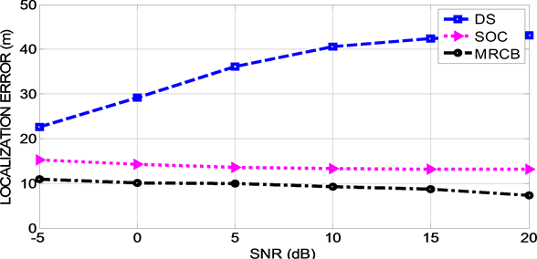
Figure 3. Point source localization error of the beamformers versus the input SNR at the simplified urban model with presence of interferences in and .
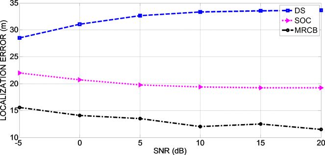
Figure 4. Point source localization error of the beamformers versus the input SNR at the Fort Benning urban model with presence of interferences in and .
In previous simulations, complete knowledge of the acoustic environment was assumed to attain the steering vector of the beamformers. It means that the localization performance of the beamforming methods is depended on the prior information of the environment to compute the steering vectors. However, there are always some uncertainties between the simulated model and the actual environment which causes error in localization of the source. In the second case, we study the beamformer performance in the presence of gradient temperature uncertainty in the simplified urban model. According to the experiments on the lowest 100 m of the atmosphere, the air can be separated into two parts: the part over the ground which the temperature gradient rate is log-linear and the second part which has a constant temperature gradient with height [31] . The minimum of the first layer height is at least 4 m in winter and 30 to 40 m in summer and the second part is a few hundred meters in height. The temperature profile uses the following equation:
(20)
where and are the absolute temperature in Kelvin at two different height and respectively and is the profile constant. Figure 5 shows the profile of the temperature versus the height. Here, 10˚C to 30˚C are chosen as a minimum and maximum temperature in the profile as shown in Figure 5 and the corresponding profile constant is 8.69. To evaluate the performance degradation due to uncertainty, the simplified urban model without any uncertainty is considered as the baseline and used to compute steering vectors. Errors due to uncertainties such as temperature gradient or were then introduced as a modification of the baseline model.
To be consistent with the previous results, the array and source are located at the same positions. The baseline case without any uncertainty (i.e. 40˚C uniform temperature) is also presented in Figure 6 for comparison purpose. Figure 6 shows that the SOC beamformer has better performance than the MRCB in presence of the temperature gradient in environment. In we have a phenomenon that causes saltation of accuracy in MRCB beamformer. This phenomenon is unknown for us and would be the target of future works. In other

Figure 5. Temperature profiles for the temperature gradient from 30˚C to 10˚C.

Figure 6. Localization error versus
SNRs, the degradation in accuracy due to uncertainty is between 0.5 m to 4 m. Additional error of the SOC beamformer is about 1 m in all SNRs because of the temperature gradient uncertainty. Table 1 shows accurate results of this experiment indicating numerically the differences between the localization error of these beamformers with and without temperature gradient uncertainty.
5. Conclusions
In this literature, we see that the MRCB beamformer has better accuracy in complex environments than SOC and DS in two simulated models. Due to more complexity of the Fort Benning urban model, the degradation in accuracy of the beamformers can also be seen even with closer distance (about 25 m) between array and source in it than in the simplified urban model. Therefore, complexity of the models plays an important role in localization error of the beamformers.

Table 1. Localization error of the SOC and MRCB beamformers with and without temperature gradient uncertainty in simplified urban model.
Secondly, the SOC and MRCB beamformers were tested with uncertainty of gradient temperature which is caused because of the difference between the numerical models and actual environments. The results show that temperature gradient uncertainty exerts more influence on MRCB than SOC. In future works, it is important to study the robustness of the beamformers to errors in the simulated models due to difference between actual environments and the models and also it is necessary to evaluate the topology effects of the source and array(s) on beamformers localization error in complex environments.
Cite this paper
Nassaji, N. and Shafieian, M. (2018) Detection of Point Sound Source Using Beamforming Technique in Complex Environments. Open Journal of Acoustics, 8, 23-35. https://doi.org/10.4236/oja.2018.82003
References
- 1. Carter, G.C. (1981) Time Delay Estimation for Passive Sonar Signal Processing. IEEE Transactions on Acoustics, Speech and Signal Processing, 29, 463-470. https://doi.org/10.1109/TASSP.1981.1163560
- 2. Weinstein, E. (1982) Optimal Source Localization and Tracking from Passive Array Measurements. IEEE Transactions on Acoustics, Speech and Signal Processing, 30, 69-76. https://doi.org/10.1109/TASSP.1982.1163855
- 3. Wang, H. and Chu, P. (1997) Voice Source Localization for Automatic Camera Pointing System in Videoconferencing. IEEE International Conference on Acoustics, Speech, and Signal Processing, Munich, 21-24 April 1997. https://doi.org/10.1109/ICASSP.1997.599595
- 4. Tsui, J.B.Y. (2000) Frontmatter and Index. Wiley Online Library. https://doi.org/10.1002/0471200549.fmatter_indsub
- 5. Richards, P.G., Waldhauser, F., Schaff, D. and Kim, W.-Y. (2006) The Applicability of Modern Methods of Earthquake Location. Pure and Applied Geophysics, 163, 351-372. https://doi.org/10.1007/s00024-005-0019-5
- 6. Huang, Y., Benesty, J., Elko, G.W. and Mersereati, R.M. (2001) Real-Time Passive Source Localization: A Practical Linear-Correction Least-Squares Approach. IEEE Transactions on Speech and Audio Processing, 9, 943-956. https://doi.org/10.1109/89.966097
- 7. Valin, J.-M., Michaud, F., Rouat, J. and Létourneau, D. (2003) Robust sound source Localization Using a Microphone Array on a Mobile Robot. Proceedings of the 2003 IEEE/RSJ International Conference on Intelligent Robots and Systems, Las Vegas, 27-31 October 2003. https://doi.org/10.1109/IROS.2003.1248813
- 8. Patwari, N., Ash, J.N., Kyperountas, S., Hero, A.O., Moses, R.L. and Correal, N.S. (2005) Locating the Nodes: Cooperative Localization in Wireless Sensor Networks. IEEE Signal Processing Magazine, 22, 54-69. https://doi.org/10.1109/MSP.2005.1458287
- 9. Ma, W.-K., Vo, B.-N., Singh, S.S. and Baddeley, A. (2006) Tracking an Unknown Time-Varying Number of Speakers Using TDOA Measurements: A Random Finite Set Approach. IEEE Transactions on Signal Processing, 54, 3291-3304. https://doi.org/10.1109/TSP.2006.877658
- 10. Cevher, V., Sankaranarayanan, A.C., McClellan, J.H. and Chellappa, R. (2007) Target Tracking Using a Joint Acoustic Video System. IEEE Transactions on Multimedia, 9, 715-727. https://doi.org/10.1109/TMM.2007.893340
- 11. Xu, Z., Liu, N. and Sadler, B.M. (2007) A Simple Closed-Form Linear Source Localization Algorithm. IEEE Military Communications Conference, Orlando, 29-31 October 2007. https://doi.org/10.1109/MILCOM.2007.4454975
- 12. Schmidt, R.O. (1972) A New Approach to Geometry of Range Difference Location. IEEE Transactions on Aerospace and Electronic Systems, 6, 821-835.
- 13. Hahn, W.R. (1975) Optimum Signal Processing for Passive Sonar Range and Bearing Estimation. The Journal of the Acoustical Society of America, 58, 201-207. https://doi.org/10.1121/1.380646
- 14. Gezici, S., Tian, Z., Giannakis, G.B., Kobayashi, H., Molisch, A.F., Poor, H.V. and Sahinoglu, Z. (2005) Localization via Ultra-Wideband Radios: A Look at Positioning Aspects for Future Sensor Networks. IEEE Signal Processing Magazine, 22, 70-84.
- 15. Asano, F., Suzuki, Y. and Sone, T. (1990) Role of Spectral Cues in Median Plane Localization. The Journal of the Acoustical Society of America, 88, 159-168. https://doi.org/10.1121/1.399963
- 16. Kulaib, A., Al-Mualla, M. and Vernon, D. (2009) 2D Binaural Sound Localization: For Urban Search and Rescue Robotics. Proceedings of the Twelfth International Conference on Climbing and Walking Robots and the Support Technologies for Mobile Machines, Istanbul, 9-11 September 2009, 423-435.https://doi.org/10.1142/9789814291279_0053
- 17. Kim, Y.-H. and Choi, J.-W. (2013) Sound Visualization and Manipulation. John Wiley & Sons, Hoboken, NJ. https://doi.org/10.1002/9781118368480
- 18. Capon, J. (1969) High-Resolution Frequency-Wavenumber Spectrum Analysis. Proceedings of the IEEE, 57, 1408-1418. https://doi.org/10.1109/PROC.1969.7278
- 19. Reed, I.S., Mallett, J.D. and Brennan, L.E. (1974) Rapid Convergence Rate in Adaptive Arrays. IEEE Transactions on Aerospace and Electronic Systems, AES-10, 853-863. https://doi.org/10.1109/TAES.1974.307893
- 20. Vorobyov, S.A., Gershman, A.B. and Luo, Z.-Q. (2003) Robust Adaptive Beamforming Using Worst-Case Performance Optimization: A Solution to the Signal Mismatch Problem. IEEE Transactions on Signal Processing, 51, 313-324. https://doi.org/10.1109/TSP.2002.806865
- 21. Boyd, S. and Vandenberghe, L. (2004) Convex Optimization. Cambridge University Press, Cambridge. https://doi.org/10.1017/CBO9780511804441
- 22. Vorobyov, S.A., Gershman, A.B., Luo, Z.-Q. and Ma, N. (2004) Adaptive Beamforming with Joint Robustness against Mismatched Signal Steering Vector and Interference Nonstationarity. IEEE Signal Processing Letters, 11, 108-111. https://doi.org/10.1109/LSP.2003.819857
- 23. Yu, Z.L. and Hwa Er, M. (2006) A Robust Minimum Variance Beamformer with New Constraint on Uncertainty of Steering Vector. Signal Processing, 86, 2243-2254. https://doi.org/10.1016/j.sigpro.2005.10.005
- 24. Gershman, A.B., Sidiropoulos, N.D., Shahbazpanahi, S., Bengtsson, M. and Ottersten, B. (2010) Convex Optimization-Based Beamforming: From Receive to Transmit and Network Designs. IEEE Signal Processing Magazine, 27, 62-75. https://doi.org/10.1109/MSP.2010.936015
- 25. Lie, J.P., Ser, W. and See, C.M.S. (2011) Adaptive Uncertainty Based Iterative Robust Capon Beamformer Using Steering Vector Mismatch Estimation. IEEE Transactions on Signal Processing, 59, 4483-4488. https://doi.org/10.1109/TSP.2011.2157500
- 26. Nai, S.E., Ser, W., Yu, Z.L. and Chen, H. (2011) Iterative Robust Minimum Variance Beamforming. IEEE Transactions on Signal Processing, 59, 1601-1611. https://doi.org/10.1109/TSP.2010.2096222
- 27. Rübsamen, M. and Pesavento, M. (2013) Maximally Robust Capon Beamformer. IEEE Transactions on Signal Processing, 61, 2030-2041. https://doi.org/10.1109/TSP.2013.2242067
- 28. Van Trees, H.L. (2002) Optimum Array Processing (Detection, Estimation, and Modulation Theory, Part IV). John Wiley and Sons Inc., New York, 3185-3201.
- 29. Cox, H., Zeskind, R.M. and Owen, M.M. (1987) Robust Adaptive Beamforming. IEEE Transactions on Acoustics, Speech, and Signal Processing, 35, 1365-1376. https://doi.org/10.1109/TASSP.1987.1165054
- 30. Gilbert, E. and Morgan, S. (1955) Optimum Design of Directive Antenna Arrays Subject to Random Variations. The Bell System Technical Journal, 34, 637-663. https://doi.org/10.1002/j.1538-7305.1955.tb01488.x
- 31. Geiger, R., Aron, R.H. and Todhunter, P. (2009) The Climate Near the Ground. Rowman & Littlefield.