Open Journal of Acoustics
Vol.2 No.1(2012), Article ID:17794,13 pages DOI:10.4236/oja.2012.21002
Three-Dimensional Free Vibration Analysis of a Viscothermoelastic Hollow Sphere
1Department of Mathematics, National Institute of Technology, Hamirpur (HP), India
2Department of Mathematics, Sant Longowal Institute of Engineering and Technology, Sangrur, India
Email: jns@nitham.ac.in, dksharma200513@gmail.com, sukhjit_d@yahoo.com
Received November 18, 2011; revised December 20, 2011; accepted December 30, 2011
Keywords: Toroidal; Spheroidal; Isotropic; Viscothermoelastic Vibrations; Spherical Structures
ABSTRACT
This paper concentrates on the study of the three-dimensional free vibrations in a homogenous isotropic, viscothermoelastic hollow sphere whose surfaces are subjected to stress free, thermally insulated or isothermal boundary conditions. The use of governing partial differential equations is solved into a coupled system of ordinary differential equations. The equation for toroidal motion gets decoupled from rest of the motion and remains unaffected due to thermal variations. Matrix Fröbenious method of extended power series is employed to obtain the solution. The secular equations for the existence of various types of possible modes of vibrations in the considered hollow sphere are derived in the compact form. The special cases of spheroidal and toroidal modes of vibrations of a hollow sphere have also been deduced and discussed. In order to explore the characteristics of vibrations the secular equations are further solved by using fixed point iteration numerical technique with the help of MATLAB software tools. The computer simulated results have been presented graphically for copper material.
1. Introduction
The exact three-dimensional analysis of free vibrations of elastic spherical structures is well established in [1-4]. The coupled theory of thermoelasticity proposed by Lord and Shulman [5] incorporates a flux-rate term into the Fourier Law of heat conduction and involves a hyperbolic-type heat transport equation admitting wave type thermal signals. Green and Lindsay [6] formulated temperature-rate-dependent thermoelasticity by introducing relaxation time that reckons a finite speed of heat propagation. Hetnarski and Ignaczac [7] studied the response of a semi-space due to a short laser pulse in context of generalized thermoelasticity. Buchanan and Ramirez [8] computed the free vibration frequencies for solid ellipsoids by using Ritz method. Sharma and Sharma [9] studied vibrations of a transradially isotropic coupled thermoelastic solid sphere by using matrix Fröbenius method. Neuringer [10] developed the procedure of Fröbenius method when the roots of indicial equation are complex. Several mathematical models [11,12] have been used to accommodate the energy dissipation is due to internal friction in vibrating viscoelastic solids. Moreover the Kelvin-Voigt model is one of the macroscopic mechanical models which is also used to describe the viscoelastic behavior of a material. Mukhopadhyay [13] studied the effect of thermal relaxation time on viscothermoelastic interactions in an unbounded body with a spherical cavity subjected to periodical loading. Sharma [14] investigated the propagation of waves in an infinite Kelvin-Voigt type viscoelastic plate in the context of coupled thermoelasticity.
This paper is devoted to the exact three-dimensional vibration analysis of homogenous isotropic, viscothermoelastic hollow sphere subjected to 1) stress free thermally insulated and 2) stress free isothermal conditions. The potential function technique has been employed to decouple purely shear motion which remains independent of thermal variations. Upon using separation of variable technique, the problem is reduced to a system of four ordinary differential equations. In order to obtain frequency equation as second class (spheroidal) vibrations the coupled system have been solved by using Matrix FRÖBENIUS series method. The fixed point iteration numerical technique with the help of MATLAB software tools is used to compute frequency and damping of the vibrations. The computer simulated results in respect of lowest frequency, dissipation factor, stresses, displacements and temperature change have been presented graphically of the hollow sphere.
2. Mathematical Model
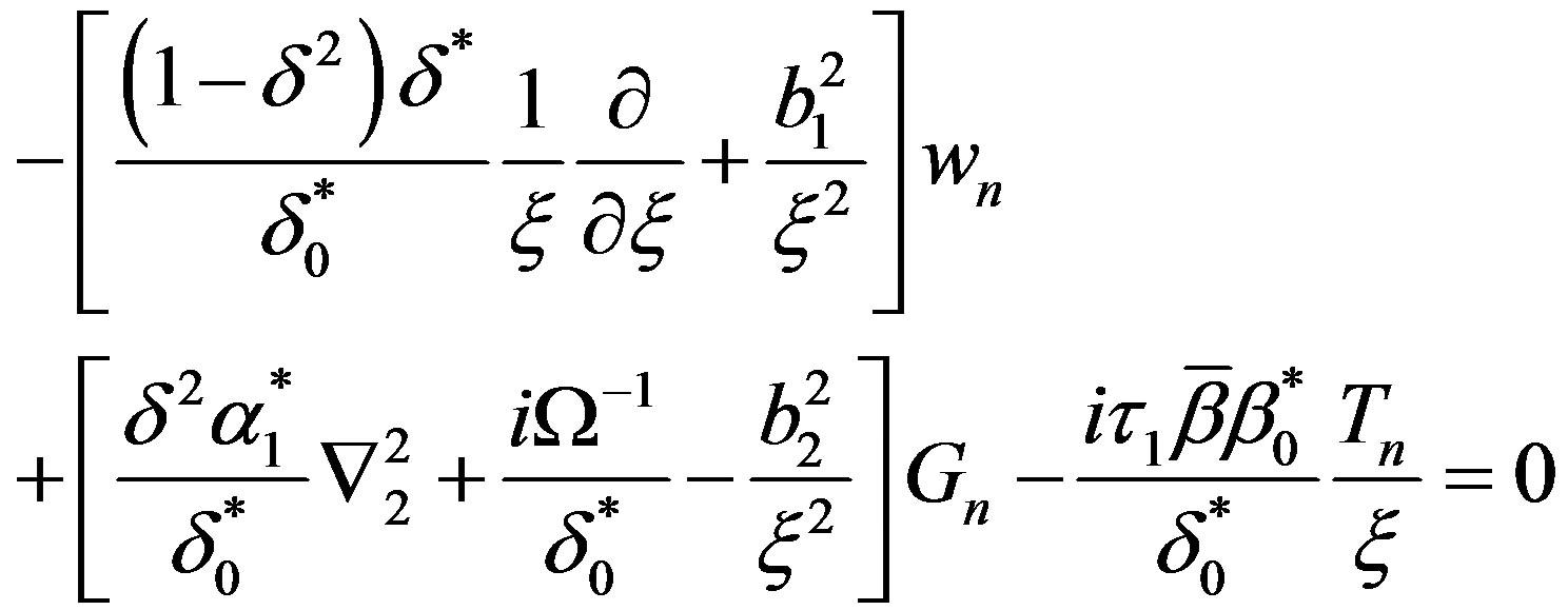
We consider a homogenous isotropic thermally conducting, viscothermoelastic hollow sphere of outer radius a and inner radius b initially at uniform temperature  in the undisturbed state. The basic governing equations of motion and heat conduction for displacement
  and temperature change
  in spherical polar coordinates
 , in the absence of body forces and heat sources, are given by [15]
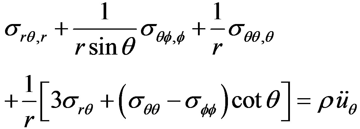 (1)
(1)
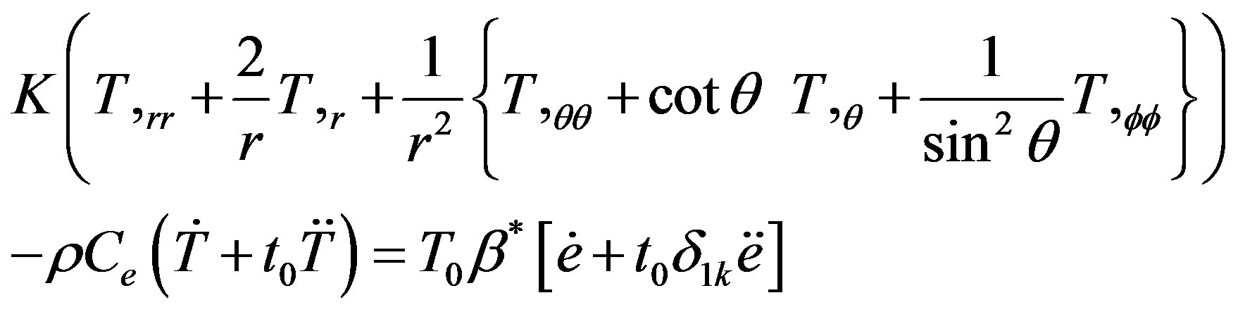 (2)
(2)
where 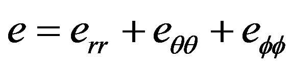


 (3)
(3)
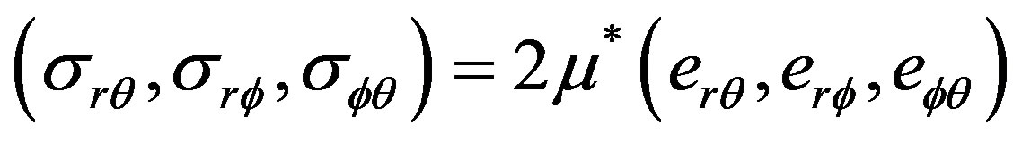
 (4)
(4)
 (5)
(5)
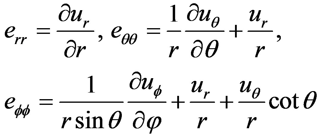
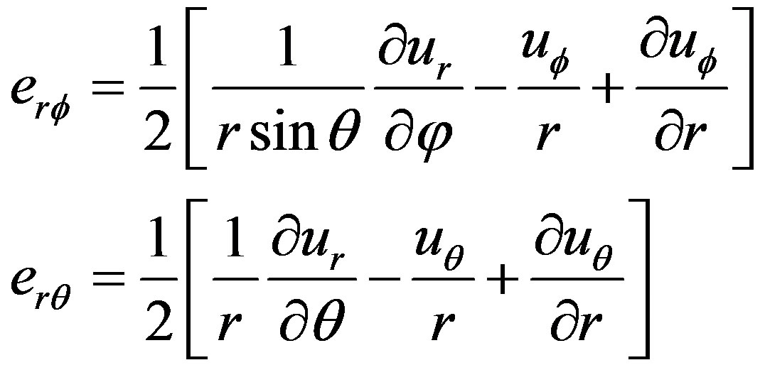
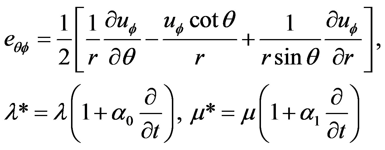
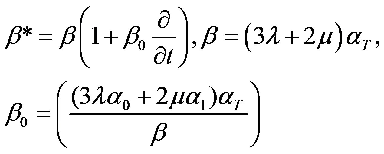
Here  and
and ,
,  are the stress and strain components, respectively;
  is the thermoelastic coupling constant,
  are the viscothermoelastic relaxation times;
  are Lame’s parameters;
  is the coefficient of linear thermal expansion;
  is mass density;
  is the specific heat at constant strain; K is the thermal conductivity;
  and
and  are the thermal relaxation times. The quantity
 ,
,  is Kronecker’s delta in which
  corresponds to Lord-Shulman (LS) and
  refers to Green-Lindsay (GL) theory of thermoelasticity. The superposed dots represent time differentiation and comma notion is used for spatial derivatives.
Boundary Conditions
We consider the free vibrations of the sphere which is subjected to stress free, thermally insulated and isothermal conditions and  (outer radius) and
  (inner radius) of the hollow sphere. Mathematically this provides us
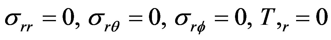 (6)
(6)
In order to simplify the model, we define following quantities
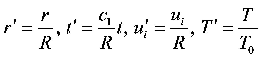
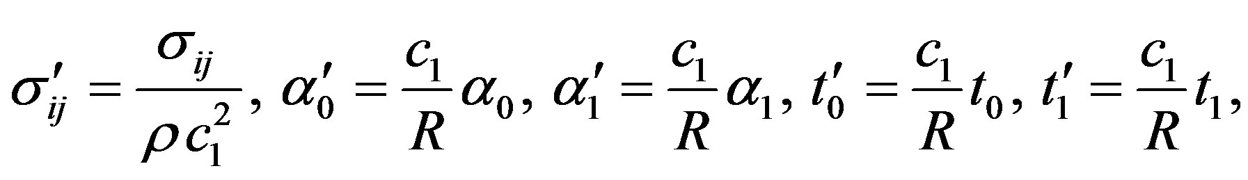
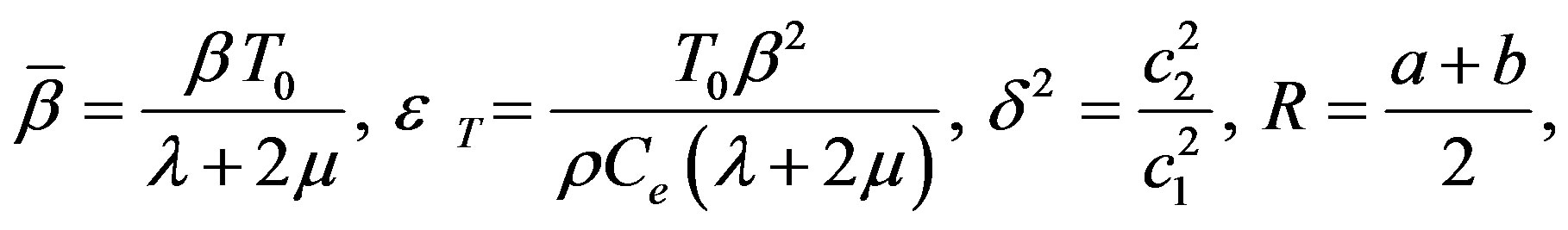 (7)
(7)
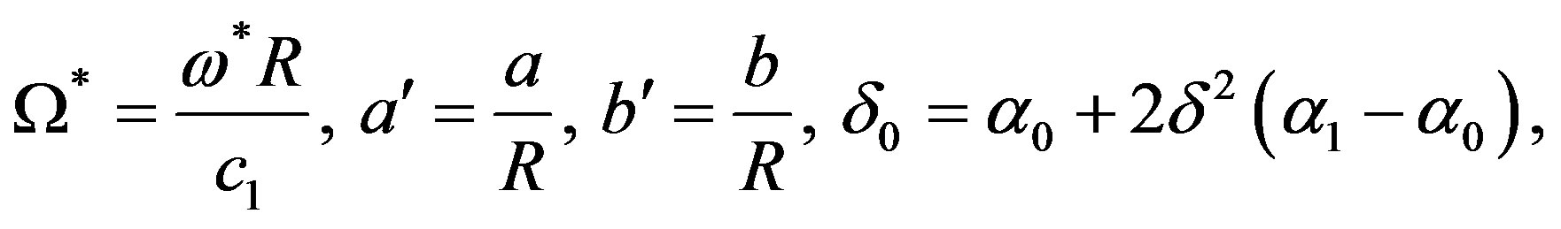
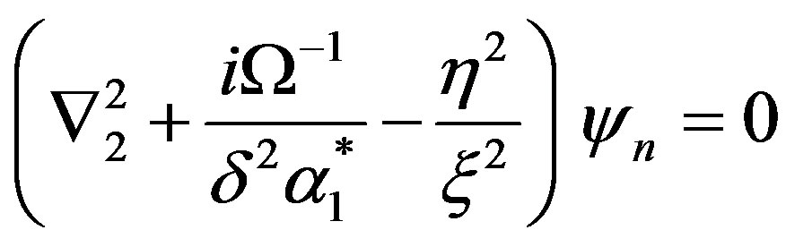
where 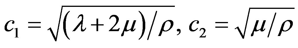 are longitudinal, shear wave velocities and
 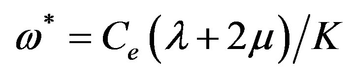 is characteristic frequency of the medium,
  is thermo-mechanical coupling constant. The primes have been suppressed for convenience.
3. Solution of the Model
In order to solve the model we introduce the potential functions  and w defined by [1]
 (8)
(8)
Upon using the Equation (8) in Equations (1) to (2), we find that  and T satisfy the non-dimensional equations
 (9)
(9)
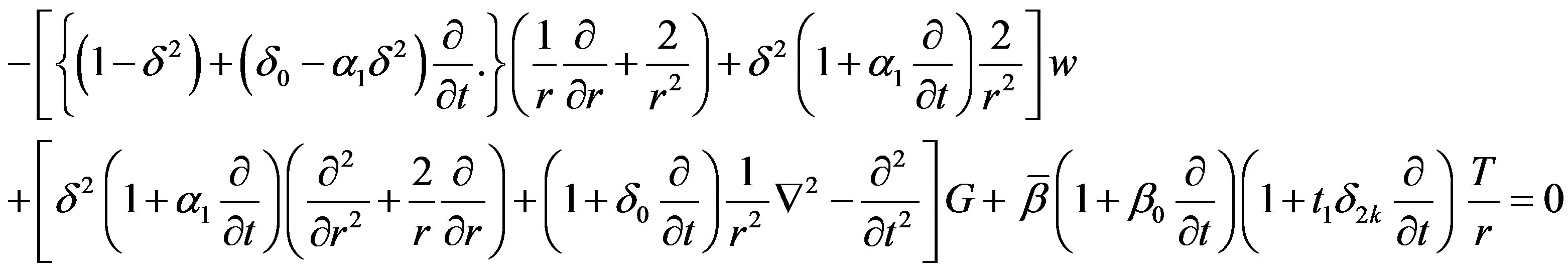 (10)
(10)
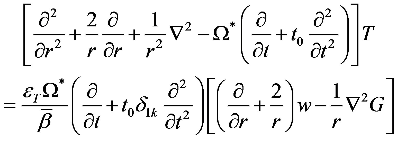 (11)
(11)
 (12)
(12)
where 
We take wave solution for the displacement functions and temperature change as under
 (13)
(13)
where 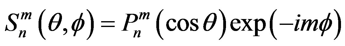 are the spherecal harmonics,
  be the associated Legendre polynomials; n and m are integers,
  ,
,  is the circular frequency. The substitution of Equations (13) into Equations (9)-(12) provides us
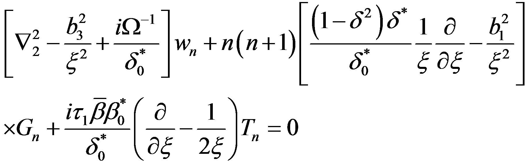 (14)
(14)
 (15)
(15)
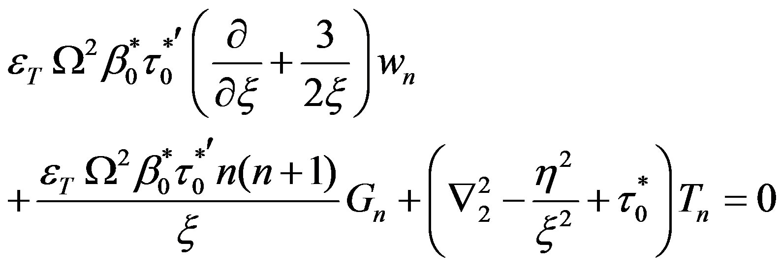 (16)
(16)
 (17)
(17)
where
 (18)
(18)
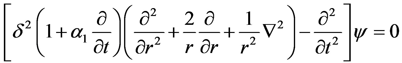
The uncoupling of Equation (17) for  from those of
  and
and  indicates the existence of two distinct classes of vibrations in the considered hollow sphere. The solution of Equation (17) for
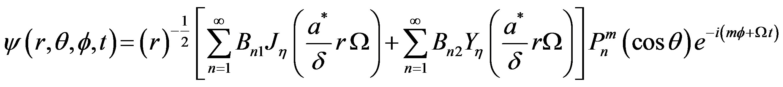
  corresponds to the toroidal modes of vibrations which remains unaffected due to thermal variations and can be discussed in the same manner as was done by Cohen [3] if viscous effects are neglected. The solution of the spherical Bessel Equation (17) is given by
 (19)
(19)
where ,
,  and
and  are arbitrary constants determined from arbitrary conditions.
3.1. Extended Power Series Method
In order to solve the coupled Equations (14)-(16), we apply Matrix Fröbenius method for the domain of consideration is . We take power series of the type
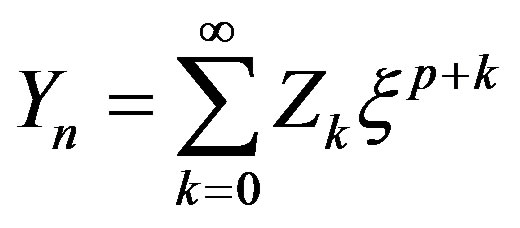 (20)
(20)
where 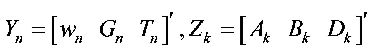
p is the eigen value and  are unknowns to be determined.
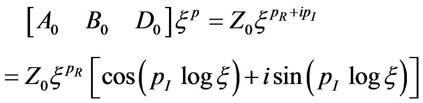
Substituting the solution (20) in Equations (14)-(16) we get the following matrix equations
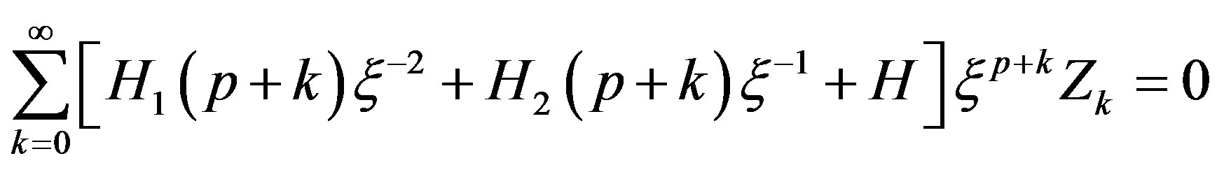 (21)
(21)
where
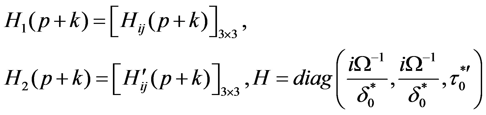 (22)
(22)
The non zero elements of the matrices  and
and  are given by
 ,
,
 (23)
(23)
where .
.
Equating to zero the coefficients of lowest powers of  (i.e.
(i.e. ) in Equation (21), we obtain
 (24)
(24)
where
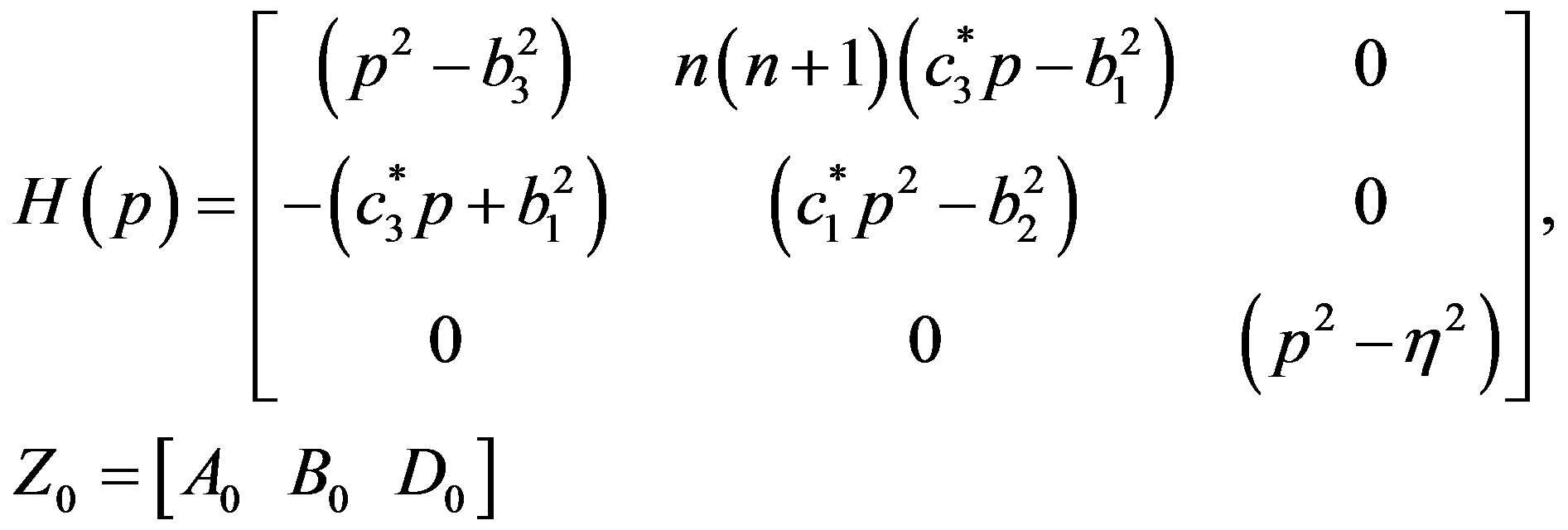
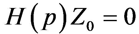
The requirement for the existence of non-trivial solution of Equation (24) leads to the following two indicial equations
 (26)
(26)
where 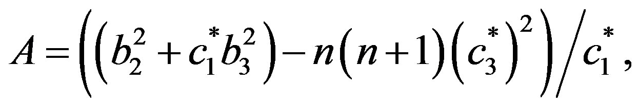
The roots of Equation (26) are of the type p = ± p (i = 1, 2, 3)
where
(27)
We designate the roots of Equation (26) as  with
with . Obviously
  are real and
  may be complex in general. If
  are complex, then leading terms in the complex series solution (24) are of the type
 (28)
(28)
In order to obtain two independent real solutions, it is sufficient to use any one of the complex root and taking its real and imaginary parts see Neuringer [10]. Moreover, the treatment of complex case is unlike that of the real roots with the advantage that the differential equation is required to be solved only once in the former case rather than twice in the later one. For the choice of roots of the indicial equations, the system of Equations (24) leads to following eigen vectors
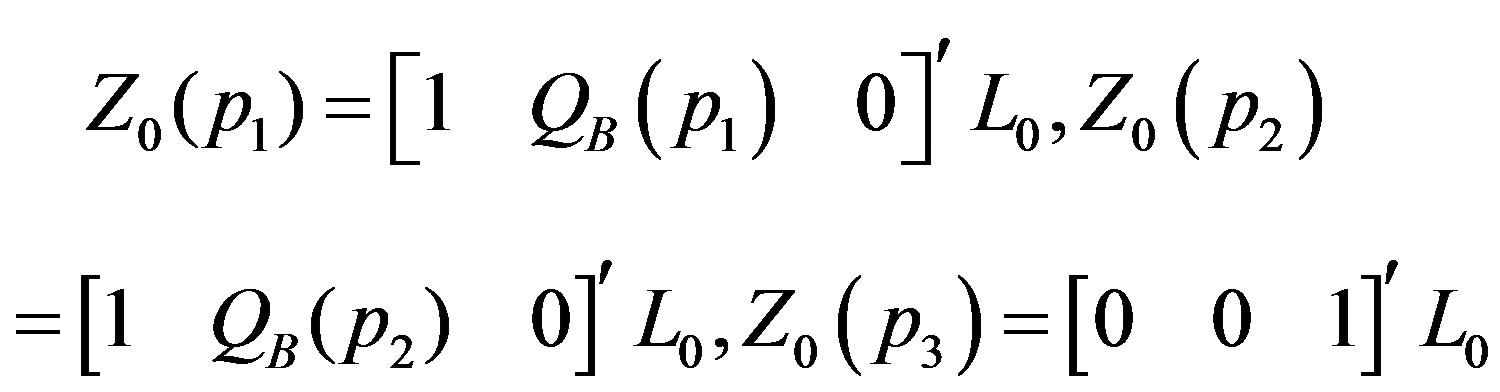
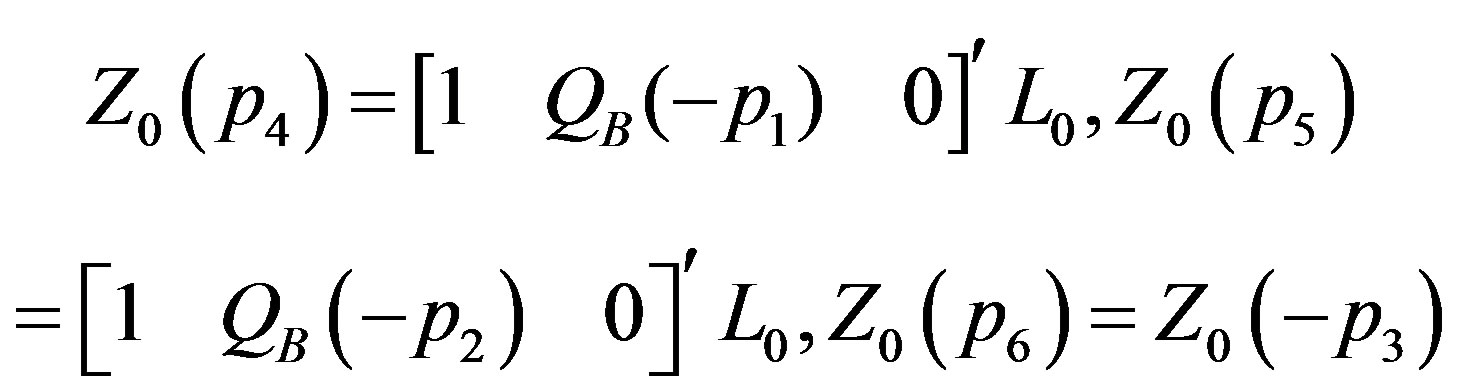 (29)
(29)
where
 (30)
(30)
and  is a constant. This suggest us to have
 (31)
(31)
where  can be written from (31) by replacing
  with
with  and again equating to zero the coefficients of next lowest degree term
 , which corresponds to
 , and using Equations (21) we obtain:
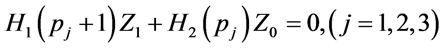 (32)
(32)
Clearly  is non-singular for each
 , therefore we have:
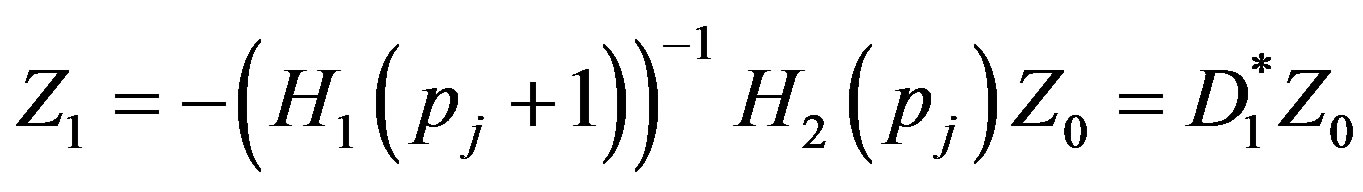 (33)
(33)
where
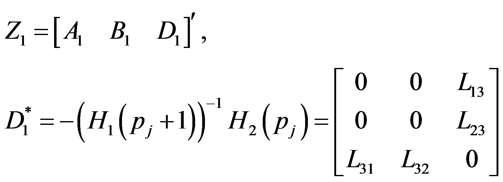 (34)
(34)
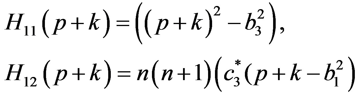
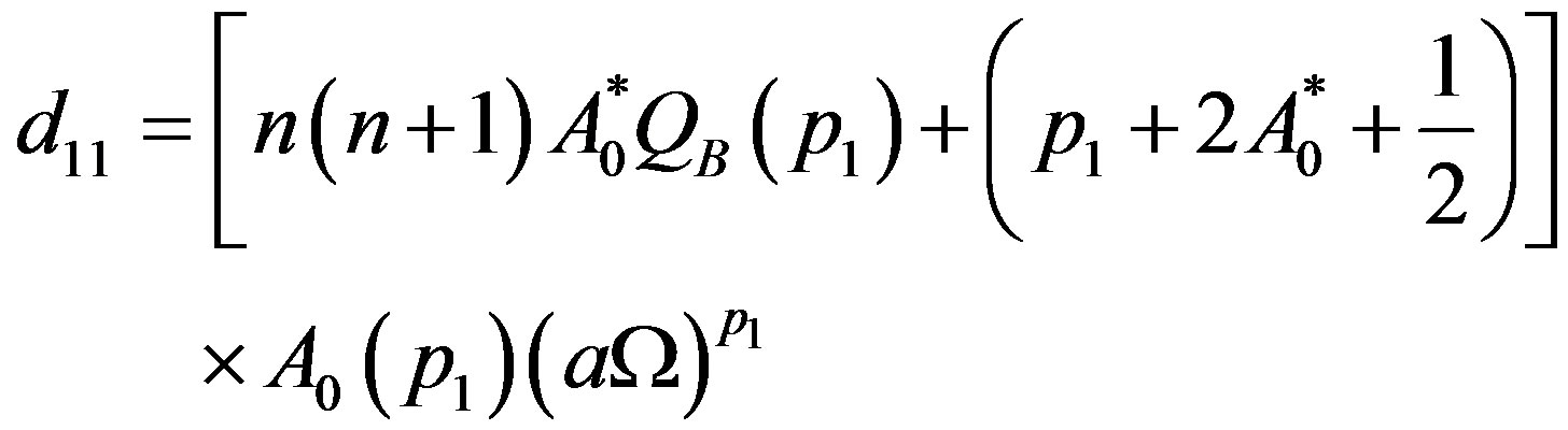
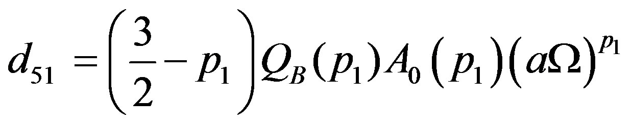
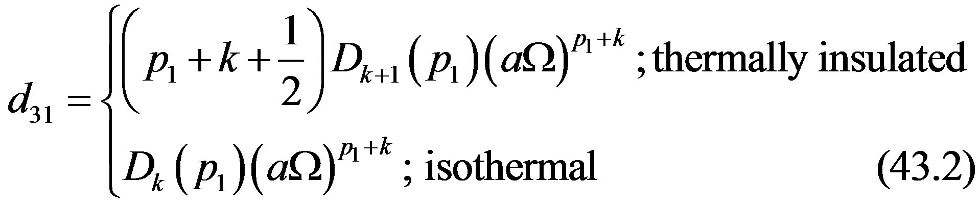
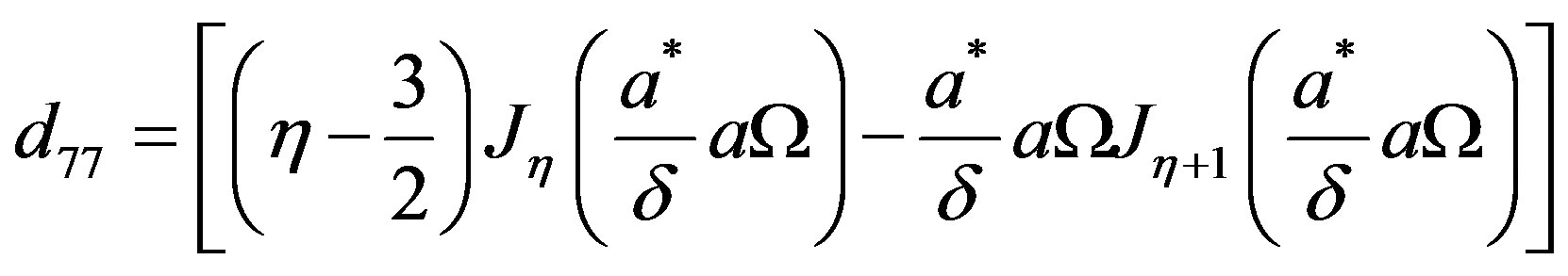
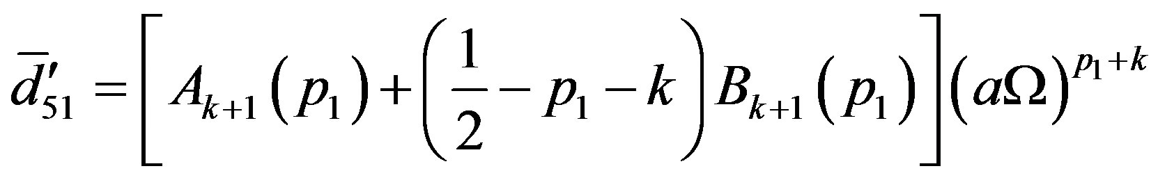
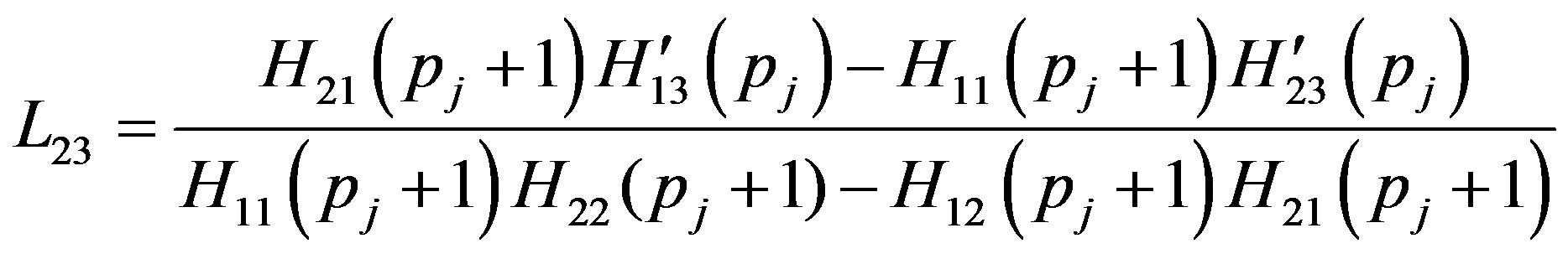
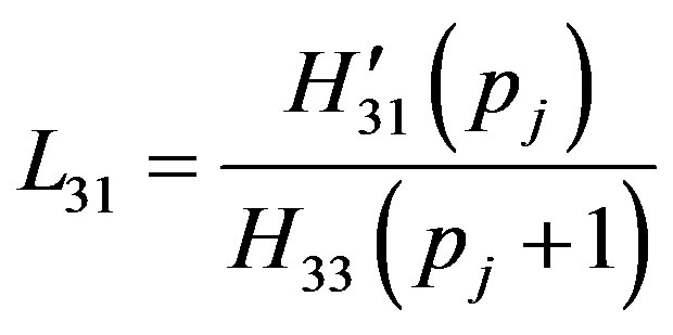
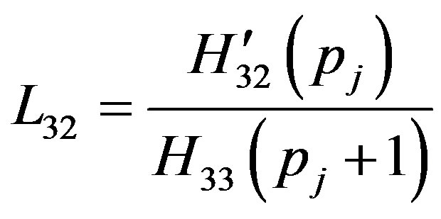
 are given by Equations (A.1) to (A.4) of Appendix. Here the matrices
  and
and  can be written from the Equations (22) and (23) by setting
  Now equating the coefficients of powers of
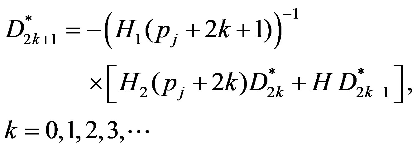
  equal to zero, we obtain following recurrence relation:
 (35)
(35)
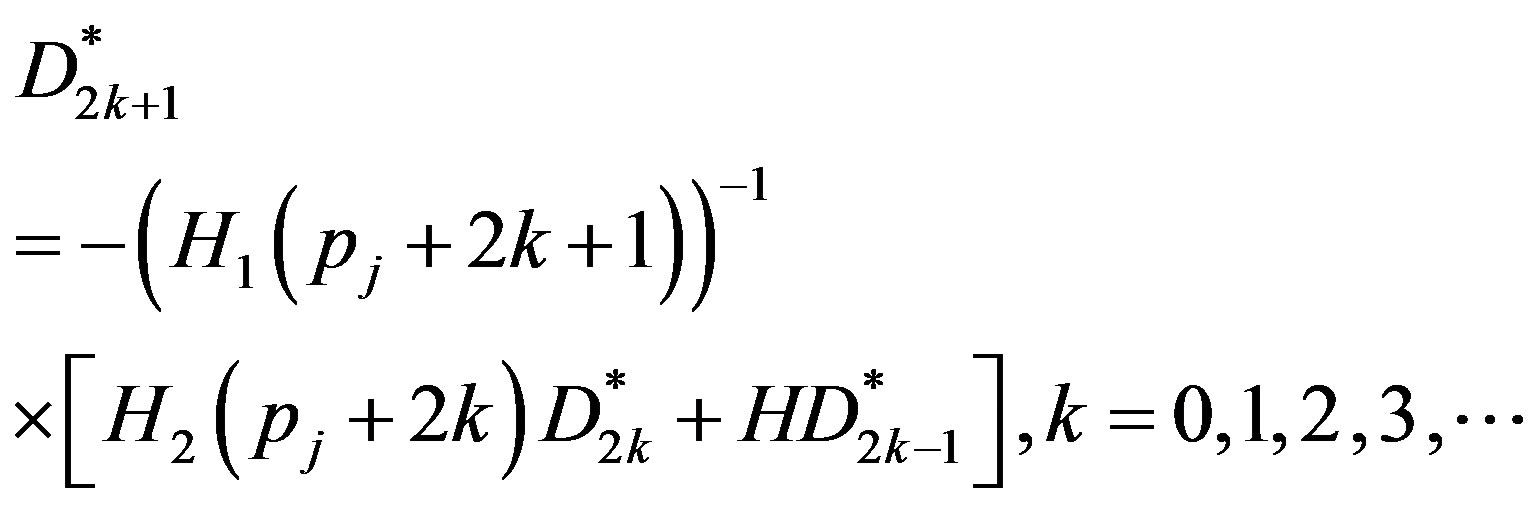
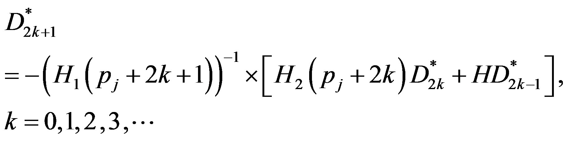
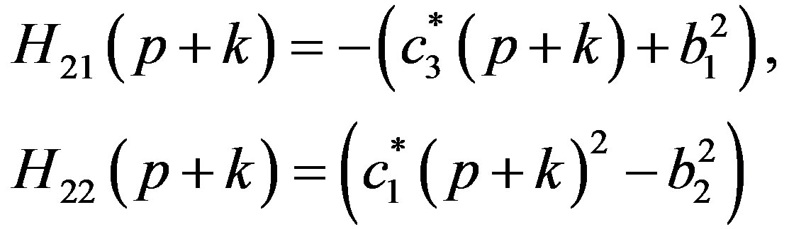
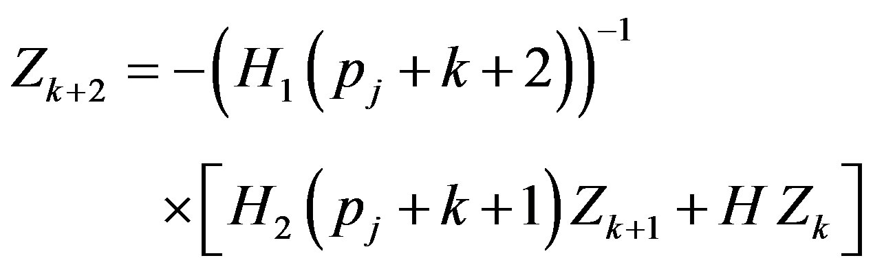
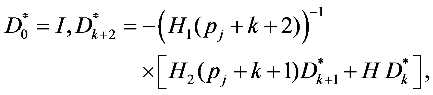
where the matrices  and H are defined in Equation (22) and (23). This implies that
 (36)
(36)
Now putting  successively, and simplifying we get
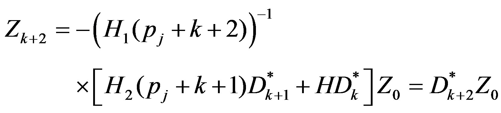
where
It can be easily shown that the matrix  has similar form to that of
  for even values of k and it is alike
  for odd values of k. Thus we have

where 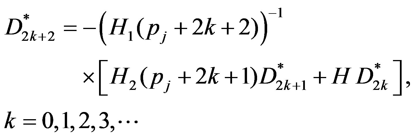
 (37)
(37)
3.2. Convergence Analysis
According to Cullen [16], in case of a matrix sequence  in
in , we have
 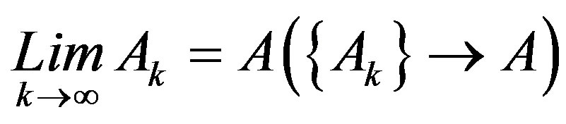 if each of the
  component sequence converges.
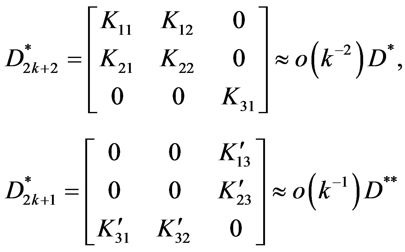
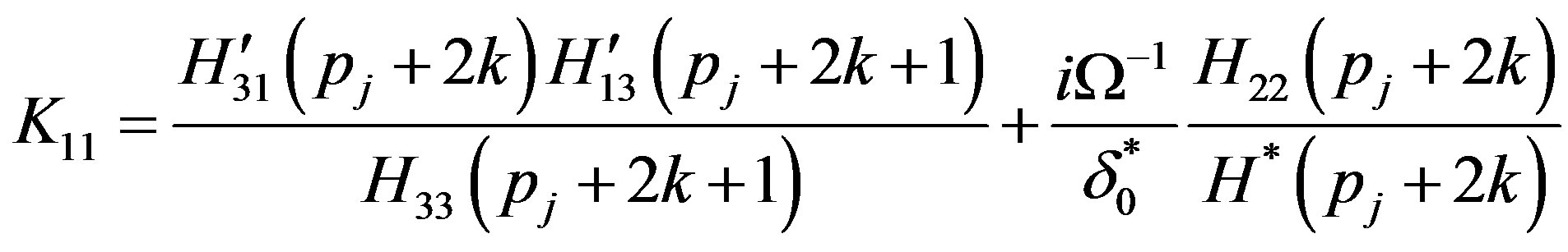
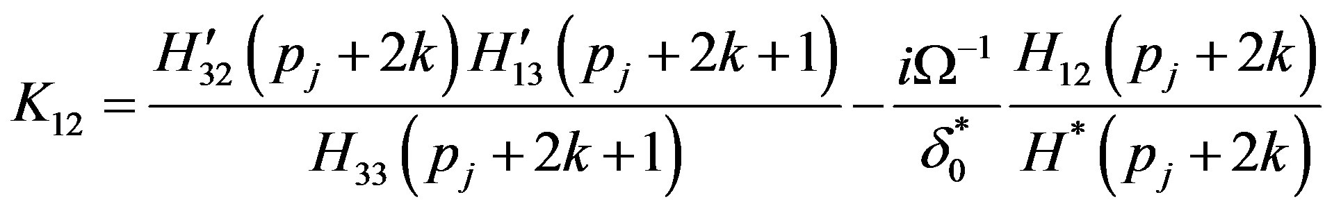
After straight forward calculations and simplifications of Equation (37) we have
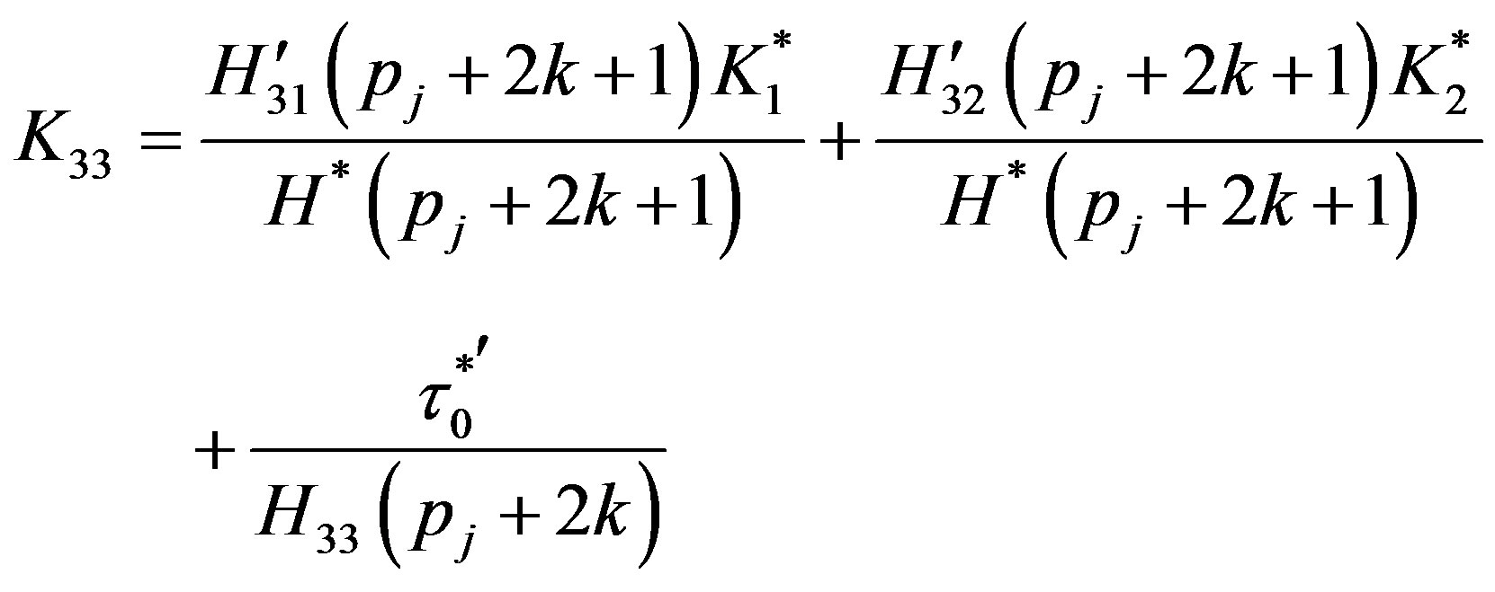
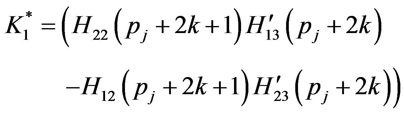
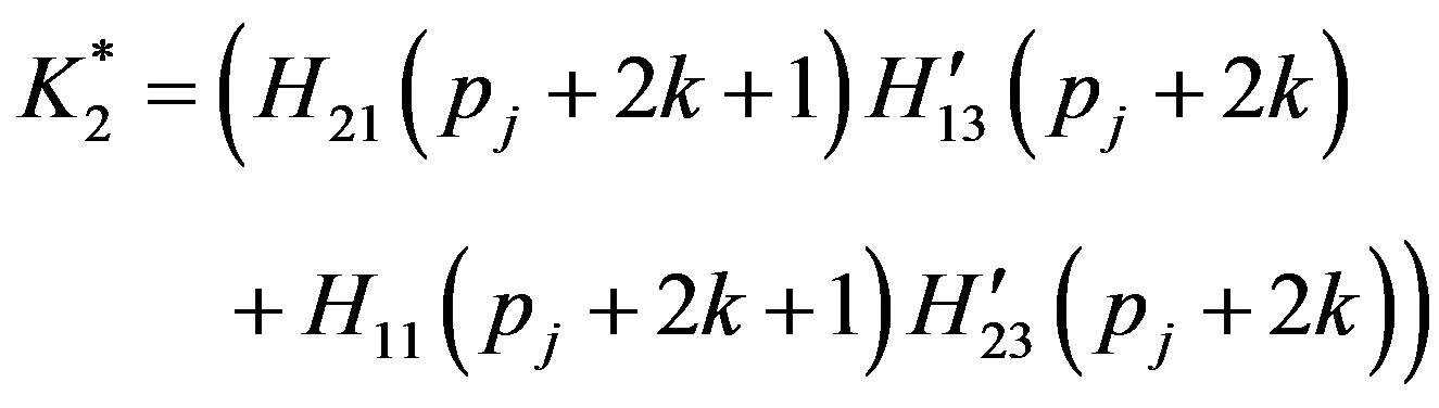
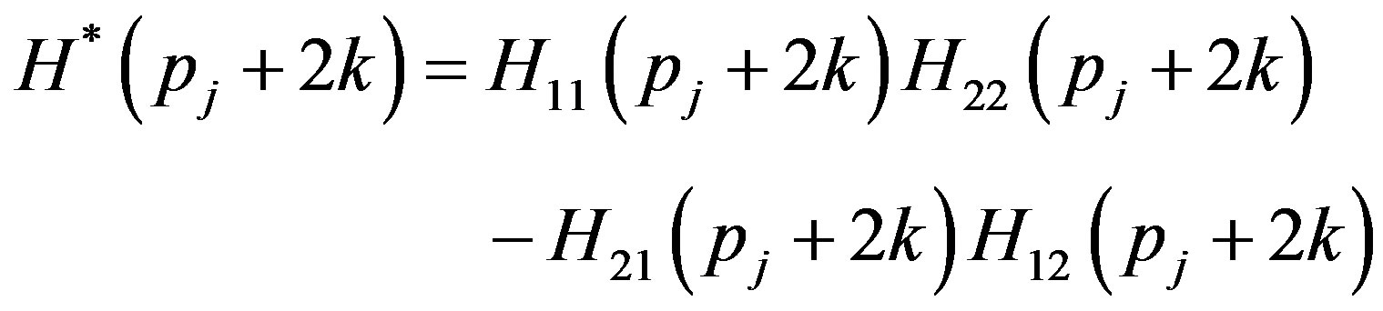
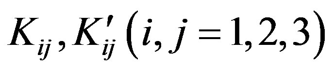 are defined by Equations (A.5)- (A.14) in Appendix.
where  and
and  is
is  null matrix. Upon using above facts, we see that both the matrices
 ,
,  , as
, as . Thus the series (20) is absolutely and uniformly convergent and hence can be differentiated term by term being analytic. Moreover, the derived series are also analytic functions. Therefore, the potential functions
  and
and  are given by
 (38.1)
 (38.2)
where 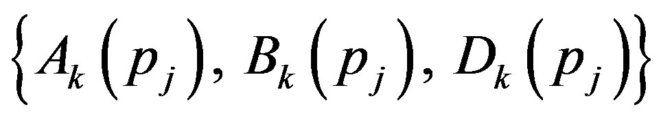 are eigenvectors shown in Appendix (A.15) corresponding to the eigenvalues
 . The unknowns
 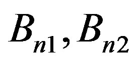 and
and  can be evaluated by four boundary conditions of hollow sphere. Displacements and stresses are obtained as
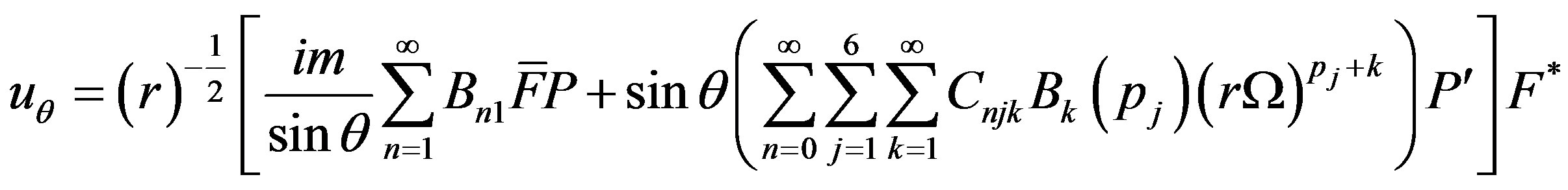
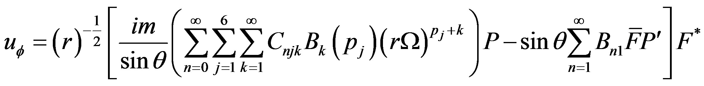
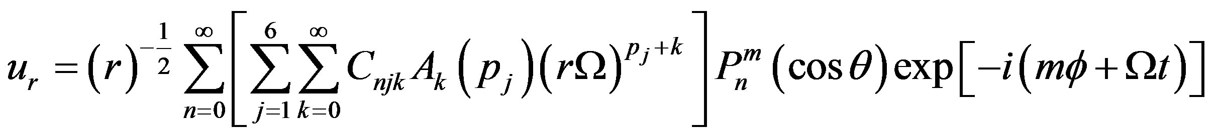 (39.1)
 (39.2)
 (39.3)
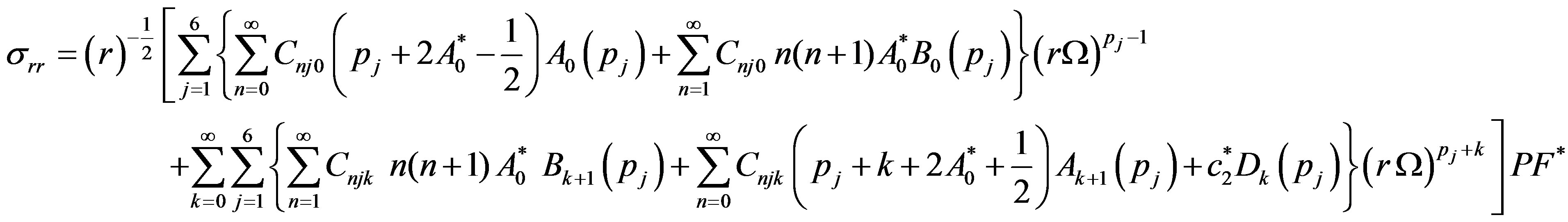 (39.4)
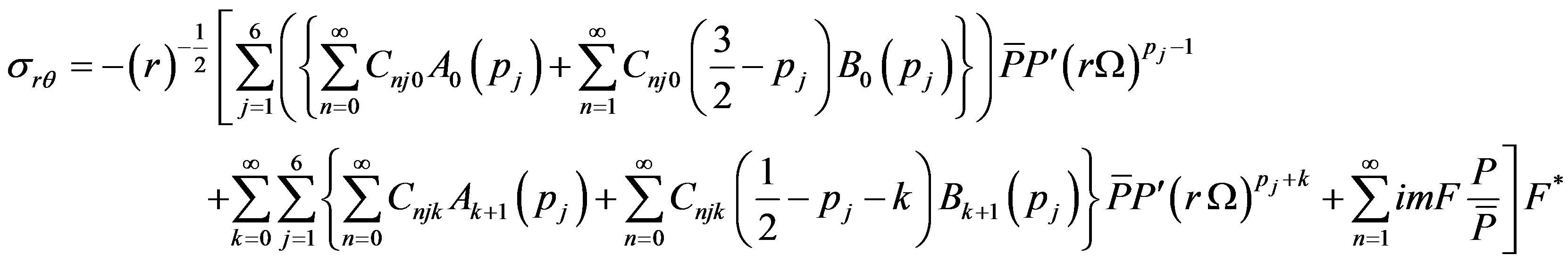 (39.5)
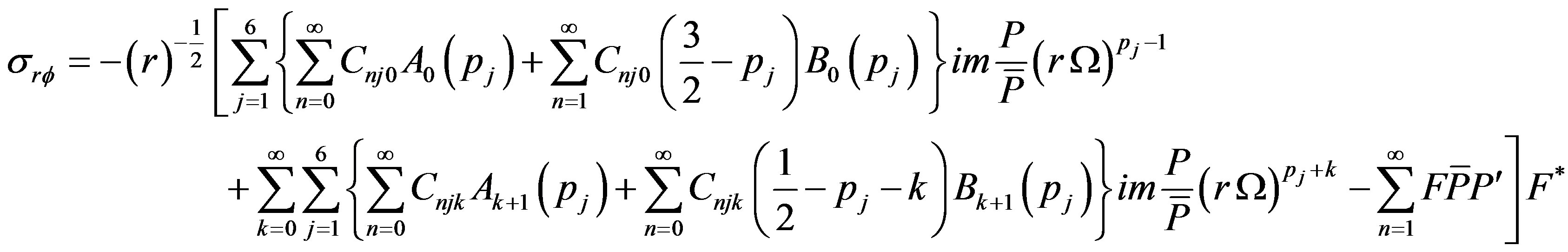 (39.6)
where 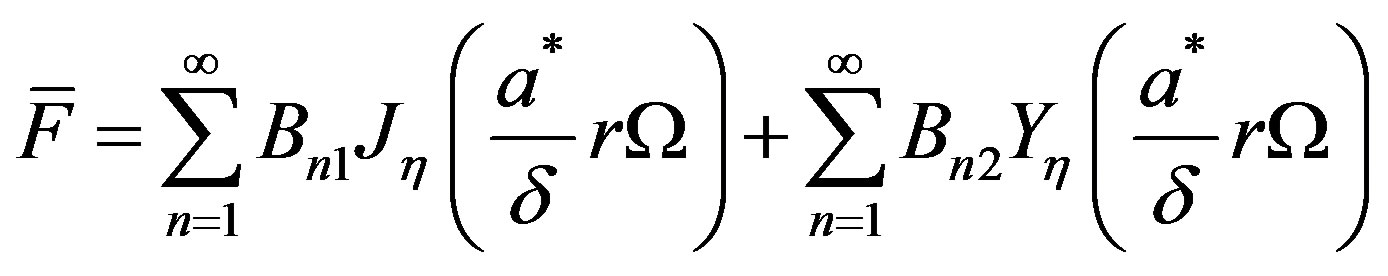
 (39.7)
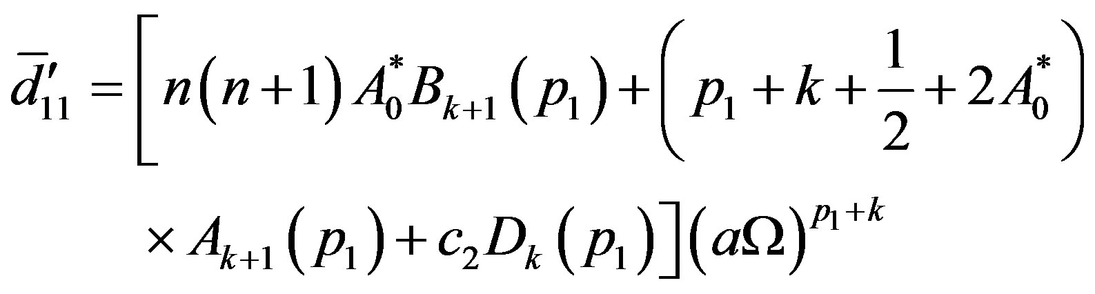
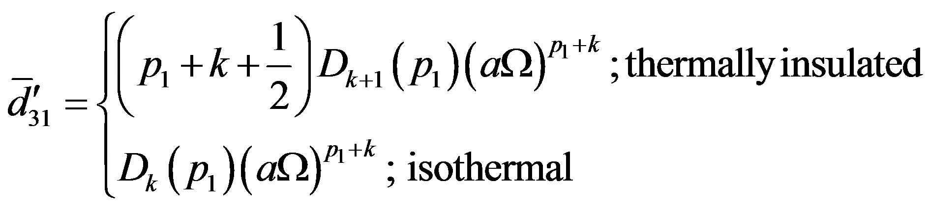
4. Secular Dispersion Relations
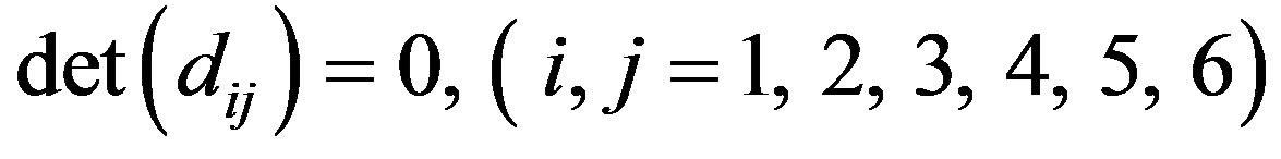
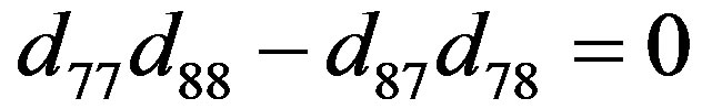
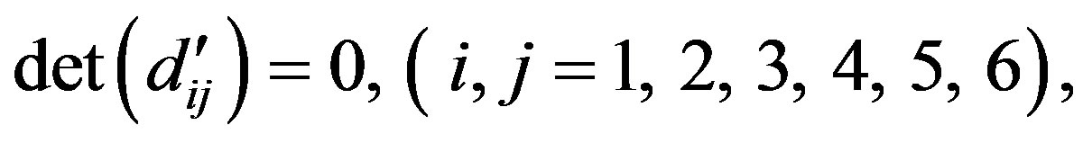
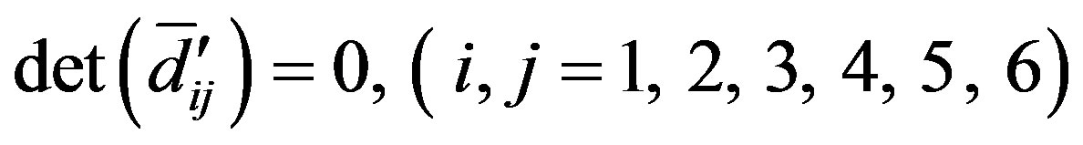
On applying the boundary conditions on Equations (6) we obtain a system of eight homogeneous linear algebraic equations which will have a nontrivial solution if and only if the determinant of the coefficients Bn1, Bn2 and vanishes. This requirement of nontrivial solution leads to a determinant equations for thermally insulated hollow sphere which further splits into two different classes of vibrations discussed below.
4.1. For Stress Free Boundary Conditions
Case 1: For  the secular equations are given as
 (40)
(40)
 (41)
(41)
 , (42)
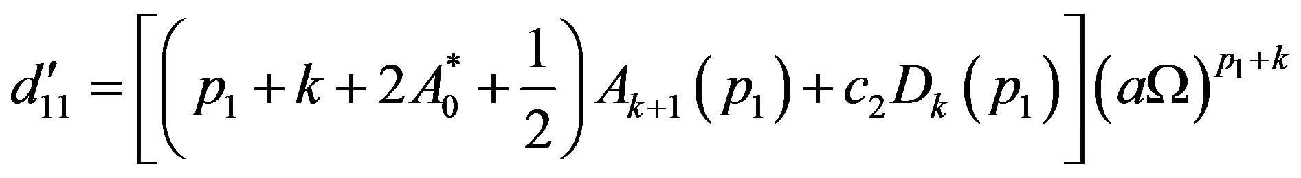
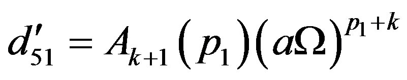
where 
 (43.1)
 (43.3)
 (43.4)
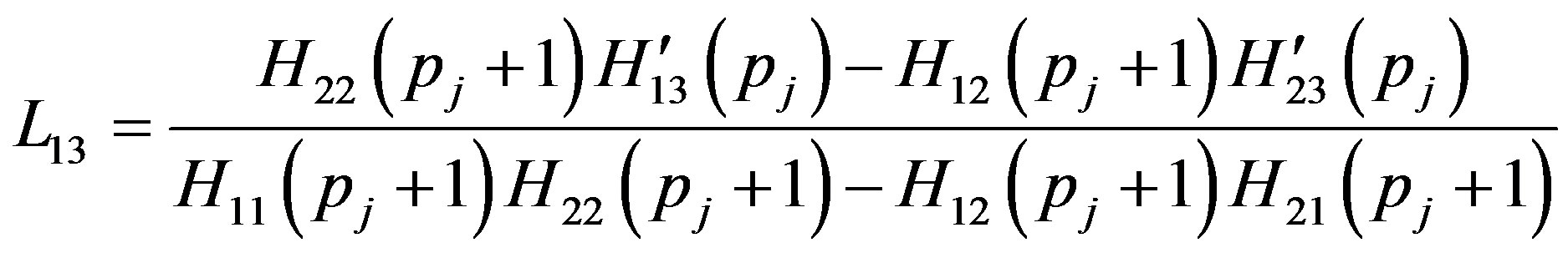
Here the elements  of Equation (40) can be written from
  by replacing
  with
with  and the elements
 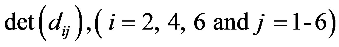 are obtained by replacing a with b. The element
  can be obtained by replacing Bessel’s function of first kind
  with that of second kind
  in Equation (43.4) and the elements
  and
and  can be obtained from
  and
and  by replacing a with b, respectively.
Case 2: For  the secular equations are obtained as
 (44)
(44)
where

The elements 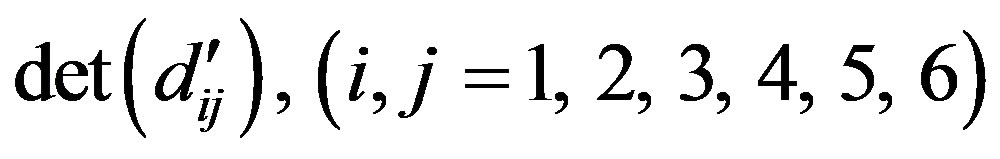 of Equation (44) can be obtained by just replacing
  in
in  with
with  while
while
 are obtained by replacing a in
 with b.
Case 3: For  the secular equations are given as
 (45)
(45)
where
The elements of 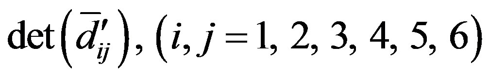 of determinant equation (45) can be obtained by just replacing
  in
in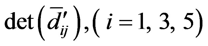 with
with
while  are obtained by replacing a in
  with b.
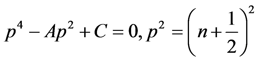
4.2. First Class Vibrations
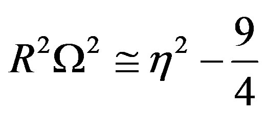
The vibrations of first class correspond to the solution of Equation (38.2) of potential function  and hence are given by Equation (41). After lengthy but straight forward calculations, the characteristic Equation (41) can be simplified by using asymptotic Expansion [3] for functions as
 (46)
(46)
where 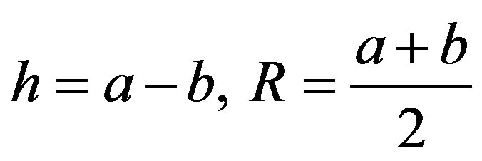 is the mean radius.
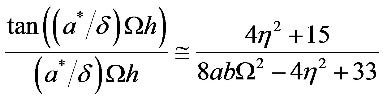
In the limiting case of the thickness h tending to zero, we obtain from Equation (46)
 (47)
(47)
These Equations (46) and (47) are of similar type reported by Cohen et al. [3] but completely agreement in the absence of viscous effect.
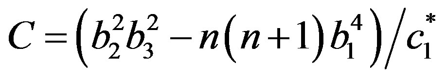
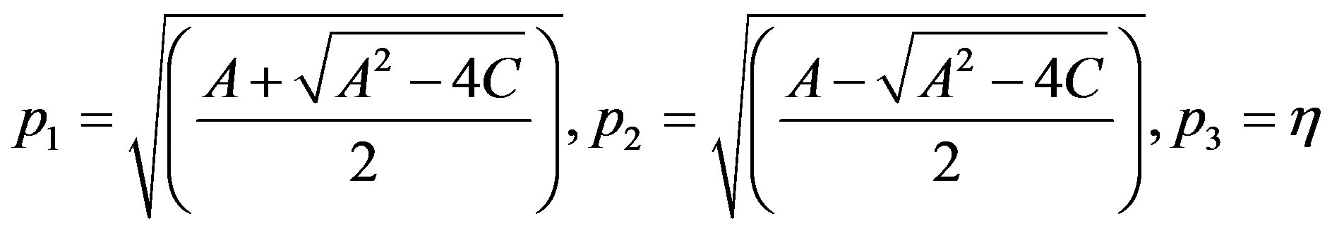
If we take 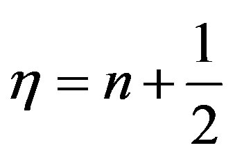 the Equation (46) reduces to
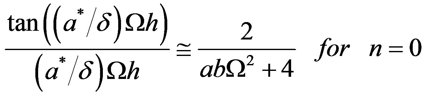 (48)
(48)
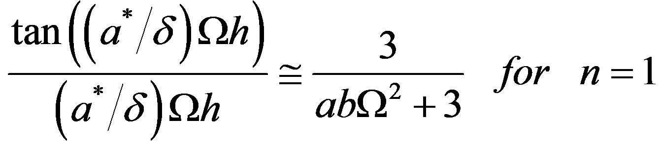 (49)
(49)
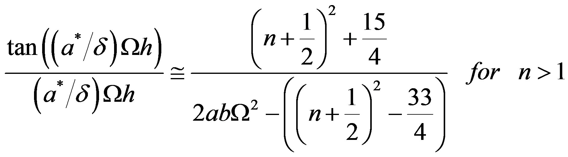 (50)
(50)
4.3. Second Class Vibrations
The secular Equations (40), (44) and (45) govern the second class vibrations called spheroidal vibrations (S-modes) for Case 1.  Case 2.
  and Case 3.
  Stress free conditions respectively.
4.4. Thermo-Elastic Hollow Sphere
If we ignore the viscous effect , then the present analysis reduces to that of generalized thermoelastic hollow sphere. In case the thermal relaxation time is zero
 , the above results reduce to those which govern the vibrations of coupled thermoelastic hollow sphere.
4.5. Viscoelastic Hollow Sphere
If thermal equilibrium is assumed to be established then , and present analysis reduces to one which governs the spheroidal and toroidal vibrations of a viscoelastic hollow sphere.
4.6. Elastic Sphere
When in addition to establishment of thermal equilibrium, the viscous effect in solid is ignored so that  , then the above analysis completely reduces to one that governs the spheroidal and toroidal vibrations of an elastic hollow sphere. In this case the results are observed to be in agreement with Cohen [3].
5. Numerical Results and Discussion
In order to illustrate the analytical developments, we propose some numerical calculations to compute lowest frequency of S-modes in the hollow sphere made of copper material. The numerical computations have been carried out for spheroidal modes of vibrations for  by using fixed point iteration numerical technique with the help of MATLAB software tools for thickness to mean radius ratio. Due to the presence of dissipation term in heat conduction Equation (2), the secular equations are, in general, complex transcendental equations and hence provide us complex values of the frequency
  and hence of
 . If we write
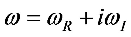 , then the lowest frequency and dissipation factor are given by
 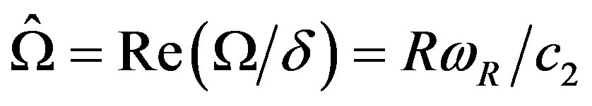 and
and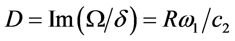 , for fixed values of n and k. The numerical computations have been done by taking sufficient number of values of the Fröbenius parameter k in order to obtain the converged values of lowest frequency
  and dissipation factor
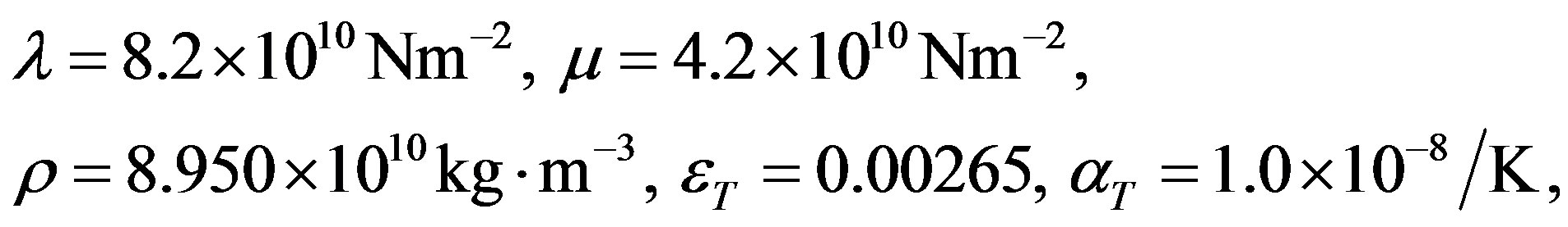
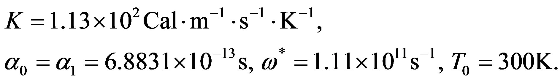
  of S-modes. The computer simulated lowest frequency, dissipation factor, displacements; stresses and temperature change have been presented in Figures 1 to 10 for viscothermoelastic (VTE), thermoelastic (TE), viscoelastic (VE), elastic (E) materials of hollow sphere. The material copper has been taken for the computation purpose as whose physical data [14] is given as
The variations of lowest frequency  and dissipation factor in a stress-free and thermally insulated hollow sphere of copper material versus degree of harmonics (n) have been plotted in Figures 1 and 2 at different values of thickness to mean radial ratio
 , where
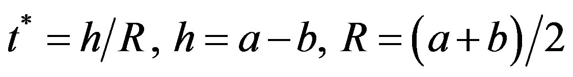 . It is concluded from Figure 1" target="_self"> Figure 1 that the lowest frequency increases with increase in degree of harmonics. It can be inferred from Figure 2 that with increase in degree of harmonics the dissipation of vibration modes go on increasing. Figure 3 the lowest frequency of toroidal vibrations has been plotted versus degree of harmonics (n) for different values of thickness to mean radial ratio
 . From Figure 3 it is revealed that with increase in the degree of harmonics the frequency of vibrations go on increasing. The trends of the profiles in Figure 3 are similar to that as reported in Ding and Chen [17]. But the dissipation factor of toroidal vibrations is very low (of the order 10–10)

Figure 1. Lowest frequency  of spheroidal vibrations versus degree of harmonics
  in (VTE) hollow sphere.
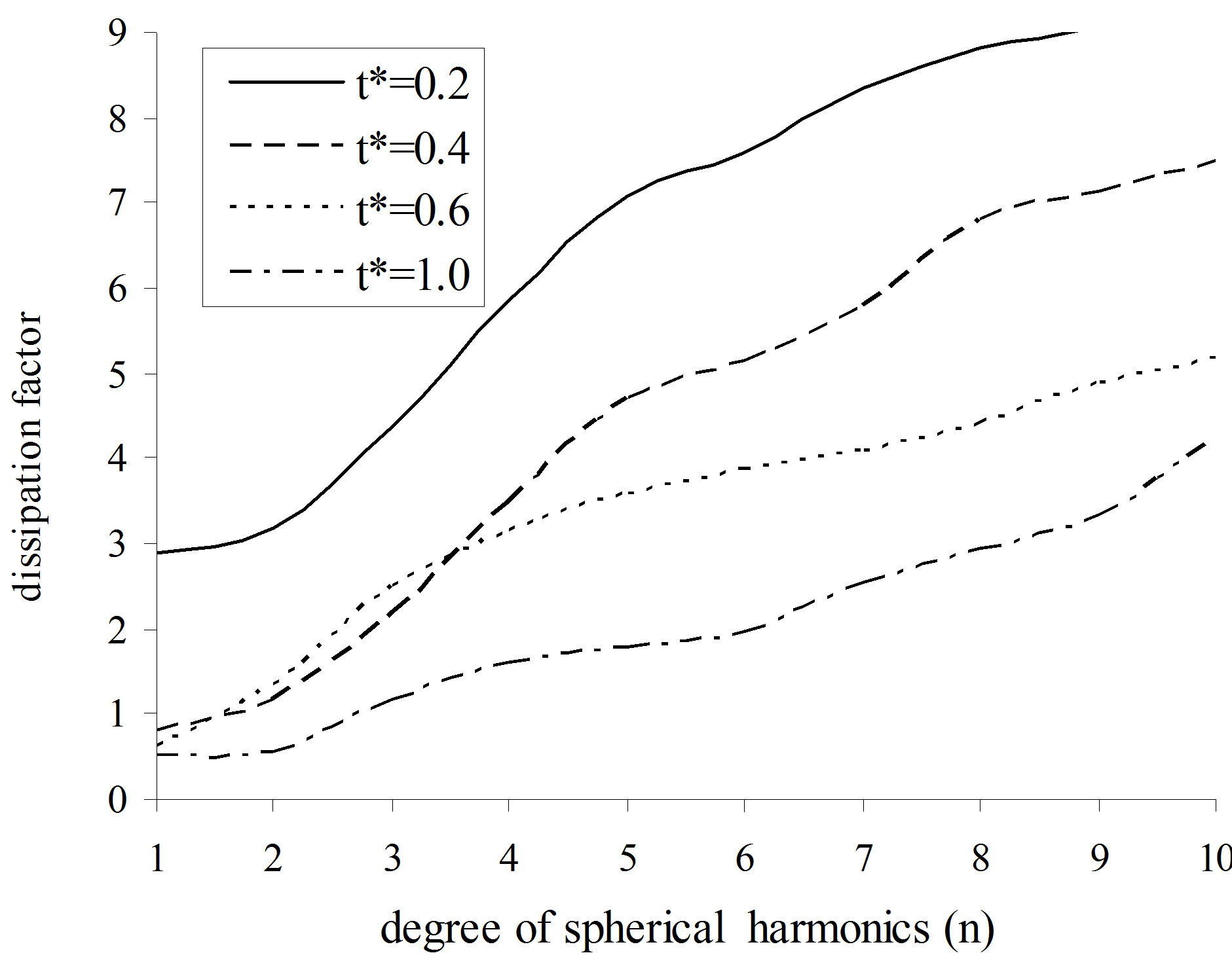
Figure 2. Dissipation  of spheroidal vibrations versus degree of harmonics
  in (VTE) hollow sphere.
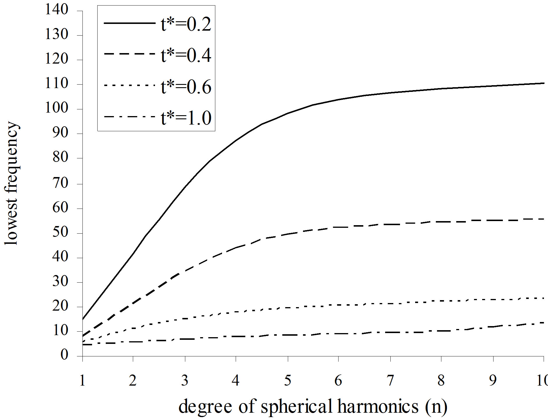
Figure 3. Lowest frequency  of Toroidal vibrations versus degree of harmonics
  in (VTE) hollow sphere
in the instant case which is negligible. From the trends of variations of lowest frequency and dissipation factor of S-mode, it is noticed that the thermal variations, thermal relaxation time and viscous nature of the material significantly affect the characteristics and behavior of spherecal vibrations and their magnitudes in contrast to that of toroidal modes which are only affected due to viscosity but not by the temperature variations as expected.
In Figures 4 to 7, the variations of temperature change (T) and stresses  versus
  i.e.
i.e.  (difference in radius and inner radius to thickness) for the modes
  and
and  have been plotted in case of stress free and thermally insulated surface of the (VTE) sphere. Figure 4 revealed that the magnitude of temperature change is though meager, but decreases with increasing values of
  from its maximum value at
  to become steady and stable at the
  in case of all the modes. It is inferred from Figure 5 that the variations of radial stress
  for modes
  initially increases and die out with increase in values of
 . But for the mode
 , the stress is of compressive nature and its magnitude vanishes with increasing values of
 . It is noticed from Figure 6 that the meridian stress
  of vibration modes
  has compressive nature and it dies out with increasing values of
 . However the mode
  has maximum variations of this quantity and its vibrations die out with increasing values of
 . Figure 7 shows that the variation of stress for mode
 . It has maximum value and its magnitude goes on decreasing with increasing values of
  to ultimately die out.
Figures 8 to 10 represent the variations of displacements  versus
  for the modes
 and
and . Figure 8 revealed that the variations of radial displacement decrease from their maximum variation
  with increasing values of
  to become stable at
  for all modes of vibrations. Figures 9 and 10 show the variations of displacements
  and
and  versus
 . The profiles of
Figure 4. Variation of temperature change  versus
  of hollow sphere.
Figure 5. Variation of stress  verses
  of hollow sphere.
Figure 6. Variation of stress  verses
  of hollow sphere.
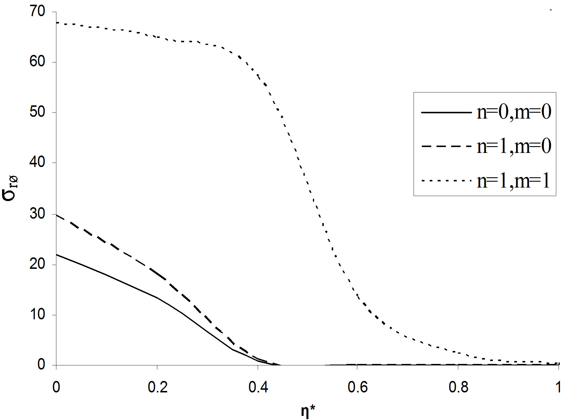
Figure 7. Variation of stress 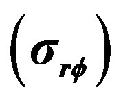 verses
  of hollow sphere.
Figure 8. Variation of displacement  verses
  of hollow sphere.
Figure 9. Variation of displacement  verses
  of hollow sphere.
Figure 10. Variation between displacement  verses
  of hollow sphere.
variations of these quantities show increasing trends with respect to increasing values of  for all the modes of vibrations.
5.1. Numerical Data/Information
Here in Table 1 shows the Comparison of lowest frequency  and Dissipation factor (D) in different media i.e. viscothermoelastic (VTE), thermoelastic (TE), viscoelastic (VE) and elastic (E) materials of hollow sphere and Table 2 has been given to check the validity of the numerical data by using t-test at fixed degree of harmonics
  for different values of thickness to mean radius ratio i.e.
  of hollow sphere.
5.2. Statistical Analysis
In this sub section we have performed some statistical analysis of computed data for lowest frequency and dissipation factor of three harmonics of spheroidal vibrations in hollow sphere of different thickness to mean radius ratio
  made from VTE, TE, VE and E materials. The t-test has been used during the analysis in order to examine the influence of thermal, viscous and both thermal and viscous, effects on the vibrations.
5.2.1. Lowest Frequency
We take two samples X and Y, where X denotes lowest frequency  of each mode of vibrations in viscothermoelastic (VTE), thermoelastic (TE) or viscoelastic (VE) hollow spheres and Y represents lowest frequency
  of elastic (E) hollow sphere. The size of the sample in each case is
  Let
Let  denote
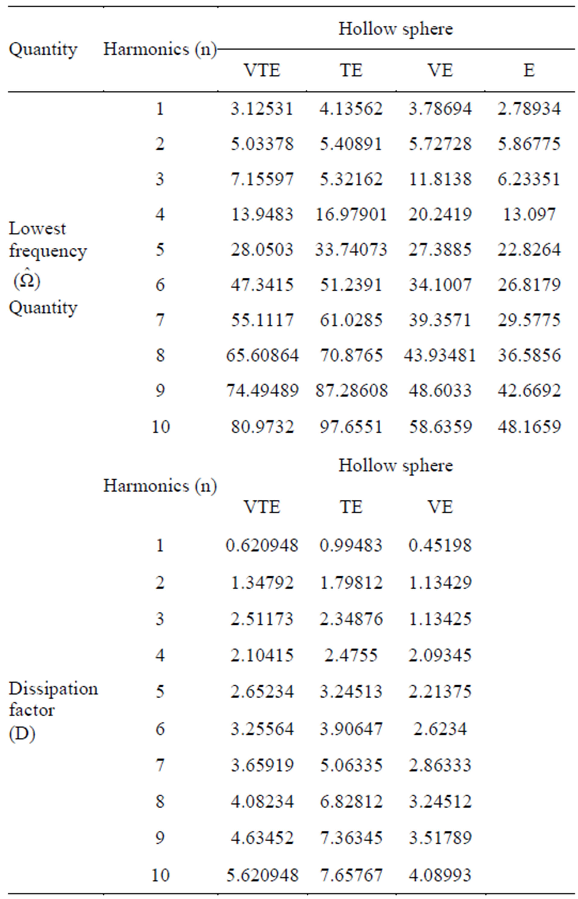
Table 1. Comparison of lowest frequency  and dissipation factor (D) of vibrations of a hollow sphere with thickness to mean radius ratio at
 .
.
mean values of the data representing to (VTE), (TE), (VE) and (E) hollow spheres, so that 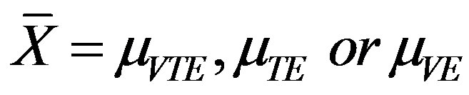 and
and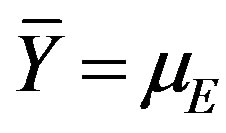 . The standard deviation
 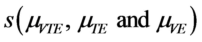 is calculated by using formula
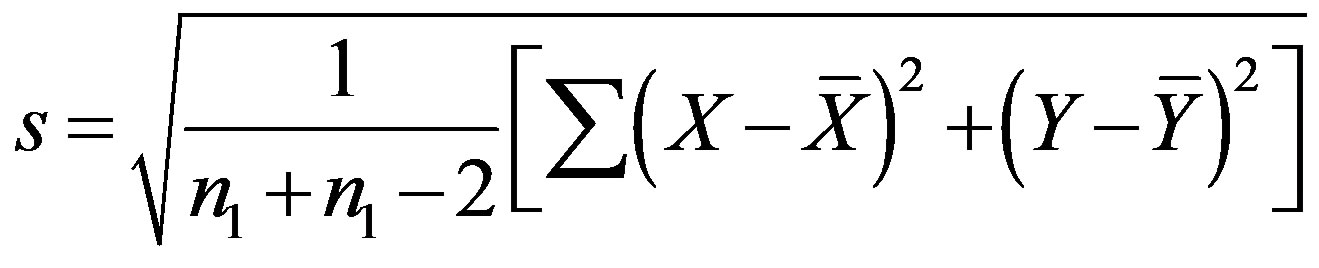 in each case for all the considered modes. In order to test the null hypothesis
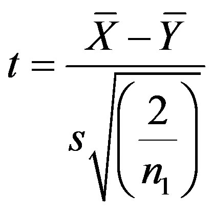
 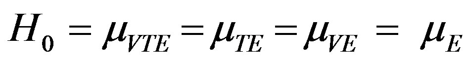 for the consistency of means of the data pertaining to each case, we use t-test in which the t-statistic is computed from the relation
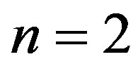
The computed values if t are given below
 :
: 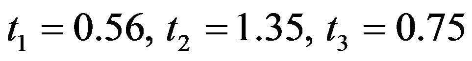
 :
: 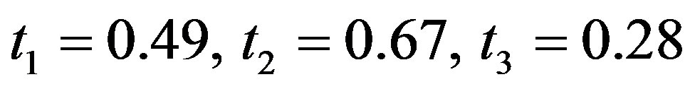
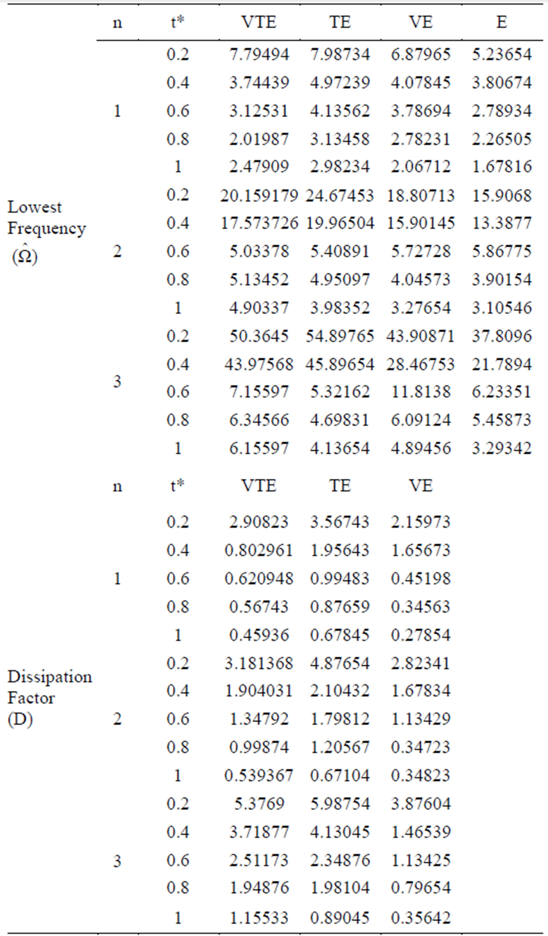
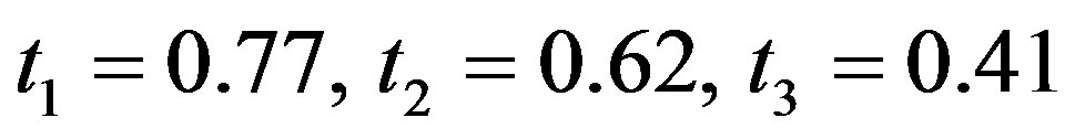
Table 2. Numerical data of lowest frequency and dissipation factor of first three harmonics  for different values of thickness to mean radius ratio
 .
.
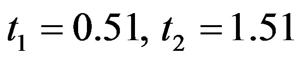
 :
: 
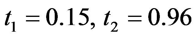
The tabulated values of t for 8 degree of freedom at  level of significance is given by
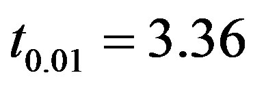 , clearly
 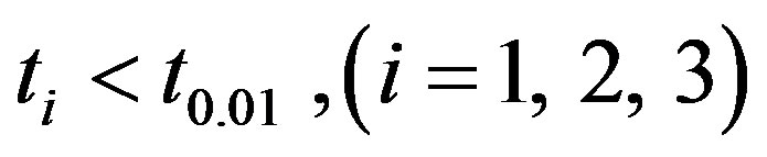 in each case and hence the null hypothesis
  is accepted at
  level of significance. Thus the numerical data is consistent.
5.2.2. Dissipation Factor
Here X denotes the dissipation factor (D) of (VTE) or (TE) hollow spheres and Y represents the dissipation factor (D) of (VE) hollow spheres. The size of the sample is again 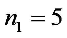 and the null hypothesis
 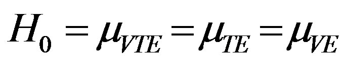 is tested for (VTE) and (TE) spheres versus (VE) one by adopting above procedure. The computed values of the t-statistic are given below:
 :
: 
 :
: 
 :
: 
Since  in each case and hence the null hypothesis
  for is accepted at
  level of significance. Thus the numerical data is consistent.
6. Conclusion
After simplifying the system of equations of motion and heat conduction of linear coupled viscothermoelasticity for a homogenous isotropic hollow sphere with the help of Helmholtz decomposition theorem, the extended power series (Matrix Fröbenius) method is successfully used to solve the resulting system of equations. It is noticed that toroidal vibrations (T-modes) get decoupled from rest of the motion and remain free of temperature variations as expected. The lowest frequency of spherical vibrations is noticed to be significantly affected due to temperature variations in a hollow sphere of copper material. This study may be useful in tribology and geophysical industrial applications.
REFERENCES
- W. Q. Chen, J. B. Cai, G. R. Ye and H. J. Ding, “On Eigen frequencies of an Anisotropic Sphere,” Journal of Applied Mechanics, Vol. 67, No. 2, 2000, pp. 422-424. doi:10.1115/1.1303803
- A. E. H. Love, “A Treatise on the Mathematical Theory of Elasticity,” Dover Publications, New York, 1944.
- H. Cohen, A. H. Shah and C. V Ramakrishan, “Free Vibrations of a Spherically Isotropic Hollow Sphere,” Acustica, Vol. 26, 1972, pp. 329-333.
- H. J. Ding, C. W. Qiu and L. Z. hong, “Solutions to Equations of Vibrations of Spherical and Cylindrical Shells,” Applied Mathematics and Mechanics, vol. 16, No. 1, 1995, pp. 1-15. doi:10.1007/BF02453770
- H. W. Lord and Y. Shulman, “A generalization of dynamical theory of thermoelasticity,” Journal of the Mechanics and Physics of Solids, Vol. 15, No. 5, 1967, pp. 299-309. doi:10.1016/0022-5096(67)90024-5
- E. Green and K. A. Lindsay, “Thermoelasticity,” Journal of Elasticity, Vol. 77, No. 1, 1972, pp. 1-7. doi:10.1007/BF00045689
- R. B. Hetnarski and J. Ignaczac, “Generalized Thermoelasticity: Closed form-solutions,” Journal of Thermal Stresses, Vol. 16, No. 4, 1993, pp. 473-498. doi:10.1080/01495739308946241
- G. R. Buchanan and G. R. Ramirez, “A Note on the Vibration of Transversely Isotropic Solid Spheres,” Journal of Sound and Vibration, Vol. 253, No. 3, 2002, pp. 724- 732. doi:10.1006/jsvi.2001.4054
- J. N Sharma and N. Sharma, “Three-dimensional Free Vibration Analysis of a Homogeneous transradially Isotropic thermoelastic Sphere,” Journal of Applied Mechanics, Vol. 77, No. 2, 2010, pp. 1-9. doi:10.1115/1.3172141
- J. L. Neuringer, “The Fröbenius method for complex roots of the indicial equation,” International Journal of Mathematical Education in Science and Technology, Vol. 9, No. 1, 1978, pp. 71-72. doi:10.1080/0020739780090110
- C. Hunter, “Visco-Elastic Waves in Progress in Solid Mechanics,” Wiley Inter-Science, New York, 1960.
- W. Flugge, “Visco-elasticity,” Blasdell, London, 1960.
- S. Mukhopadhyay, “Effect of thermal relaxation on thermoviscoelastic interactions in unbounded body with spherical cavity subjected periodic load on the boundary,” Journal of Thermal Stresses, Vol. 23, No. 7, 2000, pp. 675-684. doi:10.1080/01495730050130057
- J. N. Sharma, “Some considerations on the Rayleigh-Lamb wave propagation in visco-thermoelastic plates,” Journal of Vibration and Control, Vol. 11, No. 10, 2005, pp. 1311-1335. doi:10.1177/1077546305058267
- R. S. Dhaliwal and A. Singh, “Dynamic Coupled Thermoelasticity,” Hindustan Publishing Corporation, New Delhi, 1980.
- C. G. Cullen, “Matrices and Linear transformation,” Addison-Wesley Publishing Company, Reading, 1966.
- H. Ding, W. Chen and L. Zhang, “Elasticity of Transversely Isotropic Materials,” Springer, Amsterdam, 2006.
Appendix
The non-zero elements  of the matrix
  in Equation (34) are given by
(A.1)
(A.2)
 (A.3)
(A.3)
 (A.4)
(A.4)
The non-zero elements  and
and  of the matrix
  and
and  defined in Equation (37) are obtained as
(A.5)
(A.6)

(A.7)

(A.8)
 (A.9)
(A.9)
 (A.10)
 (A.11)
 (A.12)
 (A.13)
 (A.14)
 (A.15)
where