World Journal of Engineering and Technology
Vol.03 No.04(2015), Article ID:60875,18 pages
10.4236/wjet.2015.34017
Conjunctive Use of Engineering and Optimization in Water Distribution System Design
Essoyeke Batchabani*, Musandji Fuamba
Department of Civil, Geological and Mining Engineering, Polytechnique Montreal, Montreal, Canada

Copyright © 2015 by authors and Scientific Research Publishing Inc.
This work is licensed under the Creative Commons Attribution International License (CC BY).


Received 8 September 2015; accepted 31 October 2015; published 3 November 2015

ABSTRACT
Water Distribution Systems (WDSs) design and operation are usually done on a case-by-case basis. Numerous models have been proposed in the literature to solve specific problems in this field. The implementation of these models to any real-world WDS optimization problem is left to the discretion of designers who lack the necessary tools that will guide them in the decision-making process for a given WDS design project. Practitioners are not always very familiar with optimization applied to water network design. This results in a quasi-exclusive use of engineering judgment when dealing with this issue. In order to support a decision process in this field, the present article suggests a step-by-step approach to solve the multi-objective design problem by using both engineering and optimization. A genetic algorithm is proposed as the optimization tool and the targeted objectives are: 1) to minimize the total cost (capital and operation), 2) to minimize the residence time of the water within the system and 3) to maximize a network reliability metric. The results of the case study show that preliminary analysis can significantly reduce decision variables and computational burden. Therefore, the approach will help network design practitioners to reduce optimization problems to a more manageable size.
Keywords:
Decision-Making, Genetic Algorithm, Multi-Objective, Optimization, Water Distribution Systems

1. Introduction
Water Supply involves intricate systems and components such as treatment plants, distribution systems, pumps and tanks. Water Distribution Systems (WDSs) are designed to meet actual and future water demand under a set of constraints such as minimum pressure and good water quality. However, the factors associated with the construction and maintenance of WDSs are complicated and expensive. In the actual context of highly increasing demand, cost effective design improvement alternatives need to be identified and analyzed.
Numerous WDS optimization models including complex algorithms have been proposed over the years. Such models include linear programming [1] - [5] , nonlinear programming [6] [7] , and dynamic programming [8] . In recent years, a number of evolutionary algorithms (EAs) have been introduced for optimizing the design and operation of WDSs. These EAs include genetic algorithms [9] [10] , ant colony optimization [11] , the shuffled leaping frog algorithm [12] , particle swarm optimization [13] - [15] , harmony search [16] , genetic heritage evolution by stochastic transmission [17] and differential evolution [18] [19] . Among all these EAs, the Genetic Algorithm (GA) represents the oldest and most established evolutionary algorithm that has been applied to WDSs. As it stands, plenty of options and variants of GAs have been developed: different types of selection, crossover and mutation can be found in the literature, different codings for the variables are possible, and different hybrid versions of GAs have been proposed. A recent study by Reference [20] comparing EAs for the optimization of WDSs showed the robustness of the GA compared to the other techniques in that the results obtained were less sensitive to the parameters.
Many WDS optimization models submitted in the literature are developed on a case-by-case basis, making it hard for designers to implement them on other real world WDS design problems. For example, some models tailored for Any town network [21] - [28] , Hanoi network [29] [30] , or New York Tunnels network [31] that implement a chosen network do not always represent the different scenarios faced in the real life. Any changes in the network will then lead to a new approach to be considered as no general means are available when dealing with common points that can be successfully applied to several networks. One implication to this observation is a lack of necessary tools guiding the decision-making process for any given random WDS project. Designers need documents that can help them to map out paths at least on where they can start and to provide them with some actionable insights that can be adaptable to various networks. The issues of the need for a tank, the number of tanks, the need for a pump or the number of pumps has to be addressed where applicable. This article aims to contribute to this effort by suggesting helpful insights in a step-by-step approach to deal with WDS design problems in real practice by using both engineering and optimization. The issues raised above are discussed throughout the approach and the suggestions provided here for WDS design are intended to formulate and solve an optimization problem. The aspects emphasized in this article are: 1) the demand for a preliminary analysis before the optimization step, 2) the requirement for reducing as much as possible the number and the range of decision variables, and 3) the need for generalizing the approach as much as possible. The methodology uses a genetic algorithm to solve the formulated optimization problem. The algorithm coded in C++ is coupled with the well known simulation model Epanet [32] . The design options and criteria discussed in this article are not comprehensive but engineers frequently encounter them in real practice.
The next section of this article describes the proposed approach that a WDS designer can adopt to deal with the optimization problem. Results from the application of the approach on a real world case study are presented in Section 3. Finally, Section 4 offers a conclusion and a recommendation for future applications.
2. Approach
This article suggests practical steps to follow in order to achieve a given WDS design optimization problem from the formulation to the resolution. This section begins by identifying and formulating the main variables associated with the WDS design, and Section 2.2 defines the performance criteria which may be used in the optimization process. Section 2.3 then introduces the method proposed in this article to solve the formulated multi- objective optimization problem. Figure 1 gives an overview of the three steps.
2.1. Identify and Formulate the Design Options and Bounds
The objective of this section is to identify and formulate the main variables usually associated with the WDS design. Four network components are considered to be the main sources of the design variables. Each of these components with the associated variables is described in the following subsections.
2.1.1. Pipes
The first variable of each pipe could be the design option. Several options may be considered depending on the

Figure 1. Steps overview of the proposed approach.
problem nature (new design, rehabilitation or network expansion). These options include: 1) cleaning, 2) lining, 3) duplicating, 4) replacing, or 5) doing nothing. The “option” variable can be modeled as an integer, ranging from 1 to the number of available options. For a new design problem, this variable can be ignored.
The second variable for each pipe is the diameter size to be used. This diameter has to be chosen in a list of discrete commercial diameters. Although this list may be extensive, it is important to reduce the variable range in order to guide the optimization process toward a reasonable solution space. In this approach, a diameter is computed to be the upper limit for the diameter size. This diameter (Dsup) is based on a maximum velocity Vmax imposed by the designer. The maximum water demand Qmax for a single time step ∆t has to be computed based on the loading scenarios data (see Section 2.2.1). The upper limit diameter (Dsup) is then given in Equation (1) where Qmax and Vmax are expressed in SI. Dsup can be interpreted as the minimum diameter of a pipe that would carry Qmax at a maximum velocity of Vmax. Dcom is the nearest upper commercial diameter.
 (1)
(1)
The commercial diameters have to be sorted in ascending order with a rank assigned to each size. If RDsup denotes the rank assigned to Dsup, the “diameter size” variable can be modeled as an integer, ranging from 1 to RDsup. For a network rehabilitation problem where the pipe sizes cannot be modified, this variable can be ignored.
2.1.2. Tanks
There are several variables which could be theoretically associated with tanks in WDS design optimization [33] . In practice, these variables are highly case specific. With this approach, some parameters are computed in order to guide a decision regarding the usage of tanks.
If the number of tanks is unknown, the approach suggests computing the number (Nzones) of pressure zones. According to Reference [34] , pressure zone hydraulic grade lines should differ by roughly 30.48 m from one pressure zone to the next. Based on this assumption, Nzones is given by Equation (2) where Emin and Emax are respectively the minimum and maximum node elevations of the network. The suggestion made is to provide one tank in each pressure zone, giving a number of potential tanks equals to Nzones.
 (2)
(2)
If the tank bottom elevation variable has not been predetermined, the designer needs to set the bounds on this variable for the optimization process in order to reduce the search space. The recommended bounds are provided in each pressure zone in Equation (3) and Equation (4) based on the elevation of the pressure zone that the tank will serve. In these equations,
 and
and
 are respectively the minimum and maximum tank bottom elevation in the pressure zone i;
 and
and
 the minimum and maximum node elevations of the pressure zone i; hmin with hmax the minimum and maximum allowable pressures. These bounds are computed so that the tank could give enough pressure to the highest customer and non-excessive pressure to the lowest one. The “tank bottom elevation” can be modeled as a real variable, ranging from
 to
to
 in each pressure zone.
 (3)
(3)
 (4)
(4)
Tank volume is relegated by the capacity of components such as reserves for production, emergency, fire or balancing depending on the use of the storage. A tank should basically supply the balancing reserve for useful storage. Emergency, production and fire reserves can be estimated based on local guidelines. This article offers an approach to estimate the balancing storage Bs(m3) before moving forward to the optimization step. The estimation for this reserve is based on a full time pumping during the entire extended-period simulation time. The approach has to be applied on the whole network and on the independent pressure zones in other to evaluate the balancing reserve for different tanks. Three steps are involved in the balancing storage estimation: 1) calculate the average water demand Qmoy(m3/period) which represents the uniform pumping rate along the extended period simulation; 2) compute the tank storage volume for each time period i, Si(m3/period) by utilizing the continuity principle as in Equation (5) with an initial storage S0 of zero; 3) the balancing storage is then given by Equation (6). Qi in Equation (5) denotes the total water demand (m3/period) in the period i for the considered pressure zone.
 (5)
(5)
 (6)
(6)
Evaluating the balancing reserve coupled with the uniform pumping rate is useful especially for defining if the existing pumps and tanks are sufficient or in need of upgrading. It is also important for the optimization process to reduce the number and the range of decision variables. With the estimated needed volume known, an assumption has to be made on the shape (diameter-height ratio) to set the tank diameter.
The choice in determining tank location in real-world problems can be constrained by the availability of land already owned by the water utility or by the urban texture. In order to define this potential variable, specific information is required. If several nodes are regarded potential points for a tank location in a given pressure zone, this variable for the corresponding tank can be set as an integer starting from 1 up to the set number of candidates.
2.1.3. Pumps
There are two types of variables for pumps: pump design variables and pump operation variables. For pump design, the two parameters involved are the flow and the head. The minimum required flow is Qmoy (in Equation (5)) and the minimum required head Hp.min (if head losses are not assumed) is given in Equation (7) where Esource signifies the elevation of the pumping source. The couple (Qmoy, Hp.min) has to be regarded in selecting pump curves for each pressure zone.
 (7)
(7)
For the available pump curves, it is important to compute the maximum power with the corresponding flow and head to ascertain if these curves meet the network needs or if it is necessary to combine them for this purpose. For a rehabilitation problem, these calculations help to figure out if actual pumps need to be upgraded or not.
Pump operation can be either time-based or based on threshold tank levels or both. If only time-based controls are chosen, the pump operation variables can be formulated as binary numbers corresponding to pump status (ON/OFF) in each time step. For the threshold tank levels based operation, the variables are the tank levels leading to pump switching (ON/OFF).
2.1.4. Valves
Different types of valves can be used to limit the pressure or flow at a specific point in the network. These types include pressure reducing, pressure sustaining, pressure breaker, flow control or general control valves. If valves are to be included, the decision variables could be the location and the setting. Typically, the location is imposed by the configuration of the network, leaving the setting as the only adjustable variable. For a rehabilitation problem, the existing setting may still be effective and no change would then be required.
2.2. Define and Formulate the Design Performance Evaluation Criteria
In order to evaluate the design solutions characterized by assigning values to the variables discussed in the previous section, the performance assessment metrics have to be defined. Only feasible solutions are normally desirable and among these solutions, the best ones are found in the optimization process. This section begins with discussing the design constraints to define feasible solutions before dealing with design objectives which guide the optimization process.
2.2.1. Loading Scenarios and Design Constraints
Loading scenarios with the corresponding design constraints, set by the designer, may include normal and abnormal operation conditions. For these scenarios to run effectively, the simulation must be balanced by a specified period that can be timed in an hourly, daily, weekly or any other balancing period. The hydraulic and water quality time-steps have to be selected based on the desired level of precision and the resulting computation burden. The design constraints can be measured in terms of minimum and maximum pressures provisioned at demand nodes for each time step within the design balancing period. Depending on the designer requirements, it is possible for many other constraints to develop. Handling constraints compels that a penalty function is used, so that infeasible solutions are penalized depending on their level of infeasibility, while feasible solutions come up with a penalty score of zero. Each constraint violation that appears is reported in this penalty function.
2.2.2. Design Objectives
Design objectives are the functions that can be maximized or minimized in the optimization process. WDSs are normally built and operated so as to: minimize capital and operation cost, maximize water quality (by optimizing (maximize or minimize) the water quality indicator), and maximize various system reliability metrics that include environmental considerations. Based on the designer’s criteria, only one objective or a combination of several objectives may be at play. Some potential common objectives are discussed in the next subsections.
Costs: the total cost includes capital costs and operational costs. Capital costs consist of component costs of pipes, tanks, pumps, valves and other possible problem specific components. The operational costs, on the other hand, are basically associated with the system power usage during the design horizon; however, other problem specific operation costs can be present. The costs must take into account the lifetime of each component and the discount rate. The pipe costs are function to the pipe diameter and length while tank costs basically subject to the tank volume. The pump investment costs are representative to pump power and the valve costs are inherent on their diameters. These costs are problem specific and part of input data.
Water Quality: several parameters can be used to characterize the water quality: microbial growth, residual chlorine decay or hydraulic residence time. In numerical modeling, most of water quality models use the hydraulic residence time to compute different substance concentrations. This residence time which is expressed in the form of water age is used as water quality metric in the optimization process that can be defined in several ways. To account for water age impact on consumers, water age would be measured at non-zero demand nodes only while giving more weight to nodes with larger demands. The water age measure in Equation (8) includes these computations and can then be adopted in the optimization process.
 (8)
(8)
In Equation (8), WAnet refers to the network water age, WAij tells the water age at junction i at simulation time tj, kij is a binary variable defined as 1 if WAij is greater than a threshold WAth and zero otherwise, Qdem,ij points to the demand at junction i at time tj, Njunc is the number of system junctions and Ntime counts the number of simulation time steps.
Reliability: various metrics can be used to describe the network reliability. It is up to the designer to choose the most appropriate reliability metric for his specific problem. Three reliability measures are presented in this article: the network resilience, the greenhouse gas emissions (environmental reliability) and the leakage.
The Network Resilience In was introduced by Reference [35] to improve the earlier resilience index Ir introduced by Reference [36] as a way of measuring WDS reliability to account for means taken to mitigate the risk of failures. The Network Resilience incorporates the effects of both surplus power and reliable loops thus demonstrating the effect of redundancy. This index is computed for each time step i as in Equation (9) where np numbers the amount of pipes connected to a node, D shows the pipe diameter, h reveals the node pressure, Nr totals the number of tanks, Qr presents the tank outflow, Hr concerns the total head of the tank, Nb sums up the number of reservoirs, Qb expresses the reservoir outflow, Hb speaks to the total head of the reservoir, Np displays the number of pumps Qp and Hp are respectively the rated discharge and the head of the pump.
 (9)
(9)
The Greenhouse gas emissions are basically the result of the emissions associated with the energy required for manufacturing, transportation and installation of WDS components and the power usage from the operation of pumps. The designer may want to minimize these emissions for the sake of a sustainable development. The emission rates are part of the input data. A monetary value can be assigned to GHG emissions, enabling their inclusion in the total cost. However, Reference [37] recommended from the results of their study to separate these objectives in the optimization of WDS. A GHG objective has already been considered in some previous studies for the optimization of WDS [37] - [39] .
Leakage in a WDS can be the result of mechanical failure from pipes or other components and from pipe junctions or pipe walls in aging networks. According to Reference [40] , the background leakage in half-pipes linked to node i is calculated using Equation (10) where λ is a loss exponent, L the pipe length, θ the leak per unit surface of the pipe linking nodes i and j.
 (10)
(10)
2.3. Solve the Multi-Objective Optimization Problem
The objective of this section is to offer the method proposed in this article to solve the multi-objective optimization problem formulated in the previous sections. The optimization and simulation tools are introduced and then the optimization process is presented. Finally, the optimization results are to be analyzed so as to select a proper design.
2.3.1. Genetic Algorithm
Although many advanced Genetic Algorithms (GA) do exist in the literature and problem specific genetic operators could be developed, a steady state GA is used in this article and adapted for multi-objective optimization. For this purpose, a GA library called GALib [41] is employed which provides necessary tools for GA and its customization, along with its built-in operators. Since the genetic operators directly affect the performance of GAs, they must be carefully designed. A common problem that arises with GAs is to properly estimate the values of parameters. The following paragraphs discuss the selection of some GA parameters to effectively perform the optimization process. However, it is only indicative and other values can be assigned to these parameters depending on the computation time required to evaluate a single solution.
The population size has typical values between 50 and 1000 depending on the size of the solution space and the complexity of the adaptation evaluation [42] [43] . It is a critical parameter for the proper functioning of evolutionary algorithms. The population should be large enough to provide sufficient representative solution building blocks, allowing a multi-modal search to cover the search space adequately. If the population size is too small, then the algorithm is trapped in local areas of the search space (local optimum). However, if the popula- tion size is too large, then the algorithm will unnecessarily waste computing resources. Given these constraints, the population size is suggested to be set as follows: 1) if the total number of variables Nvar is less than 50, the population size can be 50; 2) if Nvar is between 50 and 1000, the population size can be Nvar; 3) if Nvar is greater than 1000, the population size can be 1000. This approach of assigning values can be realized as a working hypothesis taking into account the number of variables and fitting typical values. A sensitivity analysis can also be performed with respect to the static population size in order to choose the optimal value for this parameter.
There are different forms of stopping criteria such as the number of generations, the scoring of the best solution or the convergence of the population which could be used in a GA process. In the coded program, the number of generations is considered as the stopping criterion. The value to be assigned to this parameter depends on the problem size and the time budget for the whole optimization process. The analysis of some optimization problems reveals that the number of generations until convergence grows linearly with the problem size [44] [45] . Since the population is designed to reflect the optimization problem size, the number of generations can be taken proportionally to the population size with a factor of 10. With this approach the number of generations falls in a range between 500 and 10,000 that seem logical as a good exploration setting of the solution space. Although these values are not universal and may be subjected to sensitivity analysis, they represent a good compromise between the time budget and the convergence requirement.
In general, the mutation probability is taken to be low [42] . If the probability of mutation pm is too high, the algorithm degenerates into a random search, which is undesirable since the algorithm must evolve towards the optimal solution. Typical values of the probability of mutation are between 0.001 and 0.01 depending on the problem nature. One method is to adopt a probability of mutation inversely proportional to the population size like in the Non-dominated Sorting Genetic Algorithm II [46] . In the proposed methodology, this probability is designed not only to be within the typical range but also to be inversely proportional to the problem size. It is set as follows: 1) if the population size is less than 100, pm can be 0.01, 2) if the population size is greater than 100, pm can be the inverse of the population size. This event of assigning values can be seen as a working hypothesis taking note the population size and fitting typical values. Although the parameter setting may not be the best, it guarantees low values to achieve better overall performance.
Crossover is the primary operator that increases the exploratory power of GAs. Naturally, the crossover probability must be relatively high [42] . It is recommended that GA uses a moderate population size, a high probability of crossover and a low probability of mutation, even as the algorithm can be relatively insensitive to applied probability values. Typical values of the probability of crossover are rated between 0.5 and 1 depending on the case, although the probability of 0.9 is much used in the implementation of genetic algorithms as in the Non-dominated Sorting Genetic Algorithm II [46] . In this article, this common value of 0.9 is proposed for the probability of crossover since it has been used in previous studies to achieve better overall performance. This suggestion doesn’t prevent the user from choosing another value for this parameter or performing a sensitivity analysis but it can represent the starting point for the analysis process.
The issue of genome representation is primarily related to the encoding scheme. In general, it is hard to find an encoding method that transforms a problem so as to reduce or preserve the difficulty of the problem [42] . Although some representation may be preferred for some particular optimization problems, this parameter is not a critical factor for a proper functioning of GAs. For the genome representation, the program uses a binary-to-de- cimal genome to handle the optimization variables. This genome is an implementation of the traditional method for converting binary strings to decimal values. To use this genome, what is required is the ability to create a mapping of bits to decimal values by specifying how many bits will be used to represent what bounded numbers.
2.3.2. Epanet Solver
Epanet is executed in command mode. A series of DOS commands are introduced in the code to run the simulation and save results into a text file. The saved report is a comprehensive report and the results recorded at each time step for the different variables are: 1) demand nodes: actual demand, total head, pressure, quality; 2) reservoirs: net inflow, total head, pressure, quality; 3) tanks: net inflow, total head, pressure, quality; 4) pipes: flow, velocity, unit headloss, status; 5) pumps: flow, quality, head, status; 6) valves: flow, velocity, headloss, status. Epanet will also record the energy consumption for the simulation period.
2.3.3. Pareto Ranking
For a population (P) of solutions provided by the GA, a score has to be assigned to each single solution corresponding to its rank in (P). This rank reflects the degree of dominance of the solution in this population. The constrained optimization problem is reduced to an unconstrained optimization problem reported in Equation (11). Note the equivalence between maximizing reliability and minimizing −reliability. The sign “−” is used in the case the reliability metric chosen is to be maximized. If the designer elects a metric which is to minimize, this sign is removed. The penalty value is added to each term of Equation (11).
 (11)
(11)
In Equation (11), x refers to the set of problem variables defined earlier. Each solution to the problem is associated with an objective vector to be minimized. Given two solutions to the problem x1 and x2, x1 is said to dominate x2 if and only if F(x1) is partially less than F(x2); i.e., if and only if the conditions of Equation (12) are satisfied.
 (12)
(12)
A solution x0 is said to be Pareto optimal or efficient with regard to a set of solutions if and only if there does not exist any solution in this set dominating x0. The set of non-dominated solutions forms the Pareto front. The latter is the one analyzed by the decision-maker to choose the solution it deems appropriate.
There are various Pareto ranking methods in a given population [47] - [49] . A comparative study by reference [50] showed that reference [48] ’s method is stable and produces small errors in classification. This classification is the one used in this case to assign a rank to a solution x in P as shown in Equation (13). In this classification, the rank n of a solution x is the number of solutions that dominate x in P. The non-dominated solutions, therefore, all have the same rank of zero, while those seen as dominated solutions have ranks between 1 and k − 1, where k is the size of P.
 (13)
(13)
For this purpose, a basic dominance function was created in the program. This function takes as arguments two vectors of three-dimensional real x1 and x2. It returns a Boolean variable that is true when x1 dominates x2 according to Equation (12). Initializing the rank of x to 0, for each solution xi in P, i = 1 to k, if the function dominance (xi, x) returns true, the rank of x is incremented by one unit.
The score of each solution is set equal to its rank in the population. Also this score is to be minimized by GA. In this manner, the GA will favor non-dominated solutions in each generation, allowing for fast convergence towards the optimal solutions. A population evaluator is then created in the program for this purpose. This function evaluates and sets the score of each genome in the current population during the GA evolving process.
2.3.4. Optimization Process
The proposed program runs as follows (Figure 2):
a) The program reads the input file: this allows recording relevant information on the network such as the number of pipes, pumps, tanks or demand nodes.
b) From a), the program computes indicative parameters: upper limit diameter, pressure zones, minimum and maximum tank bottom elevations which are later called if needed.
c) The program provides the GA the form of a genome (solution) using the information recorded in a) and b) on the network configuration.
d) The GA generates a set of random genomes in the same format that has been provided in c). The number of genomes equals to the size of the population as computed earlier.
e) The program retrieves each genome, converts its contents and writes the Epanet’s input file for simulation by

Figure 2. Optimization process in the proposed approach.
the Epanet solver.
f) The program uses the simulation results from e) to calculate the values of the objective functions and the penalty associated with respect to constraints.
g) The program computes the Pareto rank of each genome from f). These ranks are retrieved by GA and measure the quality of each genome.
h) The GA uses genome scores from g) to generate a new improved population by selection, crossover and mutation.
Steps e) to h) are repeated until the stopping criterion is satisfied. The program saves the non-dominated genomes into a text file. Values of objective functions and penalty are recorded as well in the same file. These results are then analyzed by the decision-maker.
2.3.5. Results Analysis
The adoption of one solution among the candidates from Pareto front is not universal and obvious. It hinges on the decision priorities since gaining on a goal deteriorates at least one other goal and vice versa which leads to compromise from the designer.
The decision-maker (DM) may set a maximum residence time and then would reject solutions with a residence time that exceed the set time. If DM is less concerned about water quality and more demanding on reliability or total cost, his options becomes more and more limited.
Pareto front is usually composed of a small number of solutions and the choice is relatively less polemical. If the difficult choice comes with a great number of non-dominated solutions, one of multiple decision methods such as AHP (Analytic hierarchy process) can be engaged. The Pareto approach for multi-objective optimization allows for making a reasonable choice in a small space of solutions even if it may not necessarily be the best one.
3. Case Study
3.1. Network Description
A large and complex network environment was addressed in the recent Battle of the Water Networks [51] which was held at the Water Distribution System Analysis (WDSA) conference in Adelaide, South Australia.
The proposed approach this article brings is to apply the reduction of decision variables in this particular network environment as a means to increase decision effectiveness in solving network design issues. The full problem description pdf document and the associated Epanet input file can be obtained from the University of Exeter web page (http://emps.exeter.ac.uk/engineering/research/cws/resources/benchmarks/expansion/d-town.php).
A summary description of the problem is outlined in the next paragraphs.
The municipality of D-Town is in need of a design project to cope with the increased water demand of the population and a general increase in the population size that has led to a new residential district in the Eastern part of the city. The calibration and simulation of the actual network model shows that the existing infrastructure is not able to meet the forecasted demand, and therefore an upgrade of the network is warranted. Figure 3 reports the layout of the D-Town network which consists of five existing district metered areas (DMAs) requiring upgrades and the additional new zone to be designed. In total, The D-Town network consists of 399 junctions, 7 storage tanks, 443 pipes, 11 pumps and 5 valves, and a single reservoir. The optimization objectives contemplated by the water utility are to minimize capital and operational costs while minimizing greenhouse gas (GHG) emissions and improving water age.
The total cost requiring minimization is the sum of the annual capital costs and of the annual cost of pumping operations. The capital costs consist of component costs of pipes, pumps, valves, tanks and generators. The operational costs are calculated from the total system power usage under normal operating conditions based on a single design week. The electricity costs within the design week are specified according to normal peak and off- peak tariffs. The total GHG emissions include the emissions associated with the energy required for manufac- turing, transportation and installation of the new pipes and the power usage from the operation of pumps. The water age metric specified is WAnet as defined in Equation (8) with a water age threshold WAth set to 48h.
Two operational scenario types for D-Town are specified, a normal operation scenario, for which the network was subject to normal demand loadings, and an emergency scenario, representing the event of a power failure. The design constraints for the normal operating scenario are distinguished as nodal constraints for the balancing period of a single design week. At each time point within this design week, the demand nodes are required to satisfy minimum head constraints, and the tanks are required to not empty. A hydraulic time-step of 15 minutes
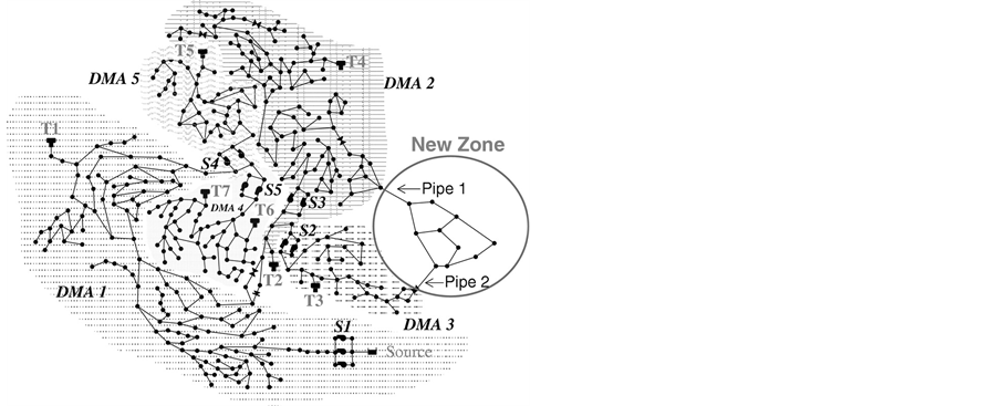
Figure 3. D-Town network layout [51] .
and a water quality time-step of 5 minutes are specified for the Epanet extended period simulations. The emergency scenarios are characterized by a power outage that can begin at any hour within the design week, and last for a duration of two hours. Within the emergency scenario, all pumps not powered by diesel generators are required to be shut down. Also constraints of minimum head for demand nodes, and non-emptying of tanks need to be met.
For the new zone, pipes are required to be sized from one of 12 diameter options (varying from 102 mm to 762 mm) for each link. The new zone is able to be connected via pipelines to either, or both, DMA2 and DMA3. For the pipe connection to DMA3, the design of a pressure-reducing valve (PRV) is permitted. The improve- ment options available to adapt the existing DMAs involved: addition of parallel pipes for all existing pipes (12 diameter options); increasing of storage volumes by one of six tank sizes (500 to 10,000 m3); addition of new pumps at the existing pumping stations (10 pump options are provided with varying head-discharge relationships); and sizing of backup power diesel generators for the pump stations (8 diesel generator options are available). For the existing DMAs, the valve settings for the existing valves are also allowed to be modified. In addition to the design options, operational pump scheduling decisions are also required to be made. As the network is specified to have a single week balancing period, the pump schedule for a single week needs to be determined. Operational controls are allowed to be either time-based, or based on threshold tank elevations.
3.2. Application Results and Discussions
3.2.1. Decision Variables and Bounds
Note that the order of the variables identified in this case study has no influence in solving the problem.
The first variable identified is the option of connection of the new zone to the existing network. This variable is modeled as an integer ranging from 1 to 5 for the five possible options which are: 1) DMA2; 2) DMA3; 3) DMA3 + PRV; 4) DMA2 + DMA3; 5) DMA2 + DMA3 + PRV.
The application of Equation (1) to the new zone gives a diameter of 102 mm for a Vmax of 3 m/s and a Qmax of 0.011 m3/s. According to the supplemental Material of reference [51] , 102 mm is the minimum allowed diameter option by the water utility. Therefore, all the diameters are set equal to 102 mm in the new zone. Consequently, there is no variable associated with the pipe design in the new zone. This reduces the problem complexity by reducing the number of decision variables.
For the existing districts, the second set of variables identified is the pipe design option for each of the 429 pipes. Since cleaning and lining are not considered as options by the water utility, these variables are modeled as integers ranging from 1 to 3 for the three possible options which are: 1) do nothing; 2) duplicate; 3) replace. The third set of variables is the diameter for each pipe in the existing districts. From the application of Equation (1) to the whole network, Dsup = 406 mm for a Vmax of 3 m/s and a Qmax of 0.379 m3/s. These variables are modeled as integers ranging from 1 to RDsup= 7 for the seven reduced possible diameter options which are (in mm): 1) 102; 2) 152; 3) 203; 4) 254; 5) 305; 6) 356; 7) 406. Reducing the range of possible values for pipe diameter limits the search space and allows for a relatively rapid convergence. Note that if the chosen pipe design option is 1 (“do nothing”) in the optimization process, this variable is ignored in the decoding process.
The application of Equations (2) to (4) gives three pressure zones for the D-Town network. Table 1 reports the computed characteristics for each pressure zone with Emin = 3.48 m, Emax = 105.63 m, hmin= 25 m and hmax = 60 m. However, in the D-Town network problem, the number of tanks, the tank bottom elevation and tank location are all fixed and the water utility does not allow for changing these properties. The only change which can be applied to existing tanks is increasing their volumes (by adopting a bigger tank diameter) if needed. In order to evaluate the need for increasing tank volumes, Equation (5) and Equation (6) are engaged in different combination of districts. The results are reported in Figure 4 and Table 2 where NZ stands for new zone.
DMA4 and DMA5 have been assessed separately because they were found to be independent from the rest of the network. Given different connection options of the new zone to the network, the DMA2 and DMA3 can be linked in some way. Note that the new zone has the same demand pattern as DMA3. So in Figure 4 and Table 2, the DMA3 includes the new zone. and Table 2 shows that the pumping station S1 is not able to provide the required flow and therefore one more pump is needed in parallel to the existing pumps in S1. All other pumping stations have a capacity greater than the required flow and don’t need upgrading. The capacity of the tank T4 is not sufficient compared to the balancing reserve which leads to the decision of adding 1000 m3 to this tank. All

Figure 4. Storage variation for different districts in D-Town network.

Table 1. D-Town Pressure zones characteristics.
Table 2. Reservoir volume and pumping capacity required for D-Town network.
other tanks have a capacity greater than the required volume and don’t need upgrading. Therefore there is no variable associated with the tank design. This reduces the problem complexity by reducing the number of decision variables.
The application results of Equation (7) to existing pumping stations are reported in Table 3. From these results, the pumping station S3 seems unable to provide the expected amount of pressure to the whole demanding nodes of DMA2. But it should be noted, however, that the elevation of the tank T4 is sufficient to cover the required pressure. In light of these findings, all the existing pumping stations and tanks are found to be adequate enough in terms of producing required pressure. For pumping operation, a decision was made to use both time based and threshold tank levels based operation. The actual operation is exclusively based on threshold tank levels but it does not guarantee the constraint of the tank being at least half full at the end of the simulation week. This would lead in this instance to favoring a manual operation policy before the optimization process. The opera-
Table 3. Pumping head required for D-Town.
tion takes into account a proper filling and emptying for tanks and the constraint of tank’s final level. The overall operation scheme is as follows: in each pumping station, each pump is switched on/off according to the connected tank threshold water levels. One pump in the pumping station S5 is switched on at the beginning of the time periods 29 and 166 regardless of the connected tank water level. The valve near the tank T2 controls the water level in this tank. Therefore there is no variable associated with pumps. This reduces the problem complexity by reducing the number of decision variables.
The locations for valves are fixed in the network and only their setting can be modified. The actual settings of PRVs are 40m for each one and from the problem description the maximum setting should be 60 m. The fourth set of variables is then the valve setting which is modeled as a real ranging from 40 to 60 for each of the 4 PRVs. Depending on the connection option of the new zone chosen in the optimization process, the decoding of the variable associated with the PRV on the pipe 2 may be ignored.
From the analysis of Table 2, the pumping stations S2 and S4 can work very well with only one pump active. So diesel generators are provided for only one pump in each of the two pumping stations. In the remaining stations, diesel generators are installed for all the pumps. In this way, the computation burden associated with power outage is reduced. Therefore there is no variable associated with diesel generators. This is another means which reduces the problem complexity by reducing the number of decision variables.
Finally, the number of decision variables identified for the D-Town network optimization problem is 863: 1 for the new zone connection, 858 for existing pipes and 4 for pressure reducing valves.
3.2.2. Decision Variables and Bounds
The optimization objectives are clearly defined by the water utility for D-Town network: minimize total cost, minimize greenhouse gas emissions and minimize water age. Although three objectives are defined, the problem can be tackled as a single-objective optimization problem by combining all the objectives in one. However, this approach doesn’t provide alternatives to enable compromise between different objectives. Therefore the multi-objective approach adopted in this article is meant to solve this problem. Given the decisions made in formulating variables, the total cost is the sum of two portions: a variable portion (pipe investment cost and pump operation cost) and a constant portion (valves, diesel generator, pumps and tanks investment cost). The constant portion is $85,636. A penalty was added for (1) a negative pressure at non demanding nodes, (2) a pressure lower than 25 m at demanding nodes and (3) a tank final level lower than the initial level. Solutions with a zero penalty are awarded to those who fully respect the design constraints.
3.2.3. Optimization and Results Analysis
In order to determine the pay-off characteristic between the total greenhouse gas emissions and water age, the genetic algorithm was run with a population size of 30 sample solutions and was allowed to run for 500 generations. Approximately 9 seconds were spent to evaluate a single solution for the formulated D-Town network problem and therefore the whole optimization process expended approximately 37 computation hours. The determination to elect a relatively low value for the population size is due to the complexity of the D-Town network and the small time steps specified for hydraulic and water quality simulations. Note that the term “-Reliability” in Equation (11) is replaced by “greenhouse gas emissions” for this problem. The power outage scenarios are only assessed at the end of the optimization process. The Pareto front identified by the GA at the end of iterations contained 11 solutions. The design values for seven of these solutions are summarized in Table 4 where V1, V45 and V47 are the three existing valves in DMA2 and N15 is the new valve on pipe 2. The seven
Table 4. Summary of design values for the seven selected solutions.
solutions are pretty similar in terms of design options and objective function values. No multiple decision method is in need here to analyze this small number of solutions. The total cost is mainly influenced by the pipe design. The number of parallel pipes (duplicated or replaced) ranges from 239 to 246. From the analysis of the results, the solution (4) is recommended for the benefits of attaining the lowest cost, greenhouse gas emissions and number of parallel pipes. The only concern ensued by this solution is amassing the highest water age metric. It is important to note, however, that all the water age values are closely ranked with each other.
The reduction of the number of decision variables and their variation range was a helpful factor in tackling this complex problem. From the competition results obtained at the conference in Adelaide, the D-Town network design if formulated purely as an optimization problem, the span of the search space could easily reach over 7500 decision variables depending on the options considered which implies that a large amount of time would be needed to solve the problem in such a situation. Through extensive preliminary analysis which resulted in uncovering four sets of decision variable groups, this greatly narrows the field to only 863 decision variables which highlights the potential of approaching complicated design issues by reducing the degree of complexity to solve the problem. It is obvious that this approach does not guarantee the global optimum as is the case for any approach intended to solve these kinds of problems. However, it does provide reasonable solutions in reasonable times to help in meeting this prominent challenge decision-makers face with real-world design problems.
Table 5 reports the objective function values found in the Battle compared to the solution (4). As can be seen, the seven authors above the solution (4) in the mentioned table found more performing solutions than the one found in this paper. The rest of the authors found a less performing solution regarding the water age objective (the five authors below the solution (4)) or the total cost objective (the last two authors). However, the optimization problem was not tackled in this paper as in the context of the Battle. The aim was to test the applicability of an overall formulation approach on a specific design problem as complex as the one addressed in the conference.
The aim of the conference, as reported in the Battle paper [51] , was not to identify the best approach to solve WDS problems. Indeed, a comparison would not be possible given the diversification of resources used by the participants [52] - [65] . Moreover, the run time was not a criterion pointed out in the competition. The aim of the conference was to identify approaches, challenges and results in solving the design problem in order to draw conclusions. A major conclusion from the conference was: there is benefit in using a combination of engineering experience and optimization methods when tackling complex real-world WDS design problem. However, the conference does not provide guiding on the aspects of approaches that can be generalized to other networks. The formulation approach proposed in this paper has the advantage of being applicable to multiple networks and it provides a competitive solution regarding the results of the conference.
4. Conclusion
A step-by-step approach for WDS design and operation has been presented, emphasizing on the need for a pre-
Table 5. Objective function values found in the Battle compared to solution 4 (data from [51] ).
liminary analysis before the optimization step, the reduction of the number and the range of decision variables, and the generalization of the design approach. In order to enlarge the scope of application of the proposed approach, some parametric equations were provided. The approach was applied to a large and complex network presented for a competition in the recent Water Distribution System Analysis (WDSA) conference in Adelaide, South Australia. The approach was able to formulate the problem with only 863 decision variables compared to the search space which could easily reach over 7500 decision variables depending on the options considered. Therefore, the proposed approach has a potential in solving WDS design problems. It can be a great guide for practitioners who are not very familiar with optimization applied to water network design and help them reduce optimization problems to a more manageable size. However, given the diversity of constraints that can be required for each network, further applications on various networks may provide insights regarding ways to improve the proposed approach. The process could very well be applicable in future especially on WDSs with more flexible terms of design constraints. It can be made to test the other aspects of the proposed approach such as tank location or tank elevation design.
Cite this paper
EssoyekeBatchabani,MusandjiFuamba, (2015) Conjunctive Use of Engineering and Optimization in Water Distribution System Design. World Journal of Engineering and Technology,03,158-175. doi: 10.4236/wjet.2015.34017
References
- 1. Alperovits, E. and Shamir, U. (1977) Design of Optimal Water Distribution Systems. Water Resources Research, 13, 885-900.
http://dx.doi.org/10.1029/WR013i006p00885 - 2. Fujiwara, O. (1990) A Two-Phase Decomposition Method for Optimal Design of Looped Water Distribution Networks. Water Resources Research, 26, 539-549.
http://dx.doi.org/10.1029/WR026i004p00539 - 3. Quindry, G., Brill Jr., E., Liebman, J. and Robinson, A. (1979) Comment on Design of Optimal Water Distribution Systems by E. Alperovits and U. Shamir. Water Resources Research, 15, 1651-1654.
http://dx.doi.org/10.1029/WR015i006p01651 - 4. Samani, H. and Mottaghi, A. (2006) Optimization of Water Distribution Networks Using Integer Linear Programming. Journal of Hydraulic Engineering, 132, 501-509.
http://dx.doi.org/10.1061/(ASCE)0733-9429(2006)132:5(501) - 5. Sherali, H.D., Totlani, R. and Loganathan, G. (1998) Enhanced Lower Bounds for the Global Optimization of Water Distribution Networks. Water Resources Research, 34, 1831-1841.
http://dx.doi.org/10.1029/98WR00907 - 6. Djebedjian, B., Herrick, A. and Rayan, M.A. (2000) An Investigation of the Optimization of Potable Water Network. 3-5.
- 7. Lansey, K. and Mays, L. (1989) Optimization Model for Water Distribution System Design = Modèled’optimisation pour la conception de systèmes de distribution de l’eau. Journal of Hydraulic Engineering, 115, 1401-1418.
http://dx.doi.org/10.1061/(ASCE)0733-9429(1989)115:10(1401) - 8. Liang, T. (1971) Design Conduit System by Dynamic Programming. Journal of the Hydraulics Division, 97, 383-393.
- 9. Simpson, A.R., Dandy, G.C. and Murphy, L.J. (1994) Genetic Algorithms Compared to Other Techniques for Pipe Optimization. Journal of Water Resources Planning and Management, 120, 423-443.
http://dx.doi.org/10.1061/(ASCE)0733-9496(1994)120:4(423) - 10. Dandy, G., Simpson, A. and Murphy, L. (1996) An Improved Genetic Algorithm for Pipe Network Optimization. Water Resources Research, 32, 449-458.
http://dx.doi.org/10.1029/95WR02917 - 11. Maier, H., Simpson, A., Zecchin, A., Foong, W., Phang, K., Seah, H., et al. (2003) Ant Colony Optimization for Design of Water Distribution Systems. Journal of Water Resources Planning and Management, 129, 200-209.
http://dx.doi.org/10.1061/(ASCE)0733-9496(2003)129:3(200) - 12. Eusuff, M.M. and Lansey, K.E. (2003) Optimization of Water Distribution Network Design Using the Shuffled Frog Leaping Algorithm. Journal of Water Resources Planning and Management, 129, 210-225.
http://dx.doi.org/10.1061/(ASCE)0733-9496(2003)129:3(210) - 13. Suribabu, C.R. and Neelakantan, T.R. (2006) Design of Water Distribution Networks Using Particle Swarm Optimization. Urban Water Journal, 3, 111-120.
http://dx.doi.org/10.1080/15730620600855928 - 14. Montalvo, I., Izquierdo, J., Perez, R. and Tung, M.M. (2008) Particle Swarm Optimization Applied to the Design of Water Supply Systems. Computers and Mathematics with Applications, 56, 769-776.
http://dx.doi.org/10.1016/j.camwa.2008.02.006 - 15. Montalvo, I., Izquierdo, J., Perez, R. and Iglesias, P.L. (2008) A Diversity-Enriched Variant of Discrete PSO Applied to the Design of Water Distribution Networks. Engineering Optimization, 40, 655-668.
http://dx.doi.org/10.1080/03052150802010607 - 16. Geem, Z. (2006) Optimal Cost Design of Water Distribution Networks Using Harmony Search. Engineering Optimization, 38, 259-277.
http://dx.doi.org/10.1080/03052150500467430 - 17. Bolognesi, A., Bragalli, C., Marchi, A. and Artina, S. (2010) Genetic Heritage Evolution by Stochastic Transmission in the Optimal Design of Water Distribution Networks. Advances in Engineering Software, 41, 792-801.
http://dx.doi.org/10.1016/j.advengsoft.2009.12.020 - 18. Suribabu, C. (2010) Differential Evolution Algorithm for Optimal Design of Water Distribution Networks. Journal of Hydroinformatics, 12, 66-82.
http://dx.doi.org/10.2166/hydro.2010.014 - 19. Vasan, A. and Simonovic, S.P. (2010) Optimization of Water Distribution Network Design Using Differential Evolution. Journal of Water Resources Planning and Management, 136, 279-287.
http://dx.doi.org/10.1061/(ASCE)0733-9496(2010)136:2(279) - 20. Marchi, A., Dandy, G., Wilkins, A. and Rohrlach, H. (2014) Methodology for Comparing Evolutionary Algorithms for Optimization of Water Distribution Systems. Journal of Water Resources Planning and Management, 140, 22-31.
http://dx.doi.org/10.1061/(ASCE)WR.1943-5452.0000321 - 21. Walters, G.A., Halhal, D., Savic, D. and Ouazar, D. (1999) Improved Design of “Anytown” Distribution Network Using Structured Messy Genetic Algorithms. Urban Water, 1, 23-38.
http://dx.doi.org/10.1016/S1462-0758(99)00005-9 - 22. Farmani, R., Savic, D.A. and Walters, G.A. (2004) The Simultaneous Multi-Objective Optimization of Anytown Pipe Rehabilitation, Tank Sizing, Tank Sitting and Pump Operation Schedules. Proceedings of the 2004 World Water and Environmental Resources Congress: Critical Transitions in Water and Environmental Resources Management, Salt Lake City, 27 June-1 July 2004, 4663-4672.
http://dx.doi.org/10.1061/40737(2004)462 - 23. Farmani, R., Walters, G.A. and Savic, D.A. (2005) Trade-Off between Total Cost and Reliability for Anytown Water Distribution Network. Journal of Water Resources Planning and Management, 131, 161-171.
http://dx.doi.org/10.1061/(ASCE)0733-9496(2005)131:3(161) - 24. Sousa, J.J.O., Cunha, M.C. and Almeida Sa Marques, J.A. (2005) Simulated Annealing Reaches Anytown. Proceedings of the 8th International Conference on Water Management for the 21st Century, Exeter, 5-7 September 2005, 69-74.
- 25. Farmani, R., Walters, G. and Savic, D. (2006) Evolutionary Multi-Objective Optimization of the Design and Operation of Water Distribution Network: Total Cost vs. Reliability vs. Water Quality. Journal of Hydroinformatics, 8, 165-179.
- 26. Prasad, T.D. (2007) Design of Anytown Network with Improved Tank Sizing Methodology. Proceedings of the Combined International Conference of Computing and Control for the Water Industry CCWI2007 and Sustainable Urban Water Management SUWM2007, De Montfort Leicester, 3-5 September 2007, 391-396.
- 27. Vamvakeridou-Lyroudia, L.S., Savic, D.A. and Walters, G.A. (2007) Tank Simulation for the Optimization of Water Distribution Networks. Journal of Hydraulic Engineering, 133, 625-636.
http://dx.doi.org/10.1061/(ASCE)0733-9429(2007)133:6(625) - 28. Prasad, T.D. (2010) Design of Pumped Water Distribution Networks with Storage. Journal of Water Resources Planning and Management, 136, 129-132.
http://dx.doi.org/10.1061/(ASCE)0733-9496(2010)136:1(129) - 29. Cembrowicz, R.G., Ates, S. and Nguyen, K.M. (1996) Mathematical Optimization of the Main Water Distribution System City of Hanoi, Vietnam. In: Blain, W.R., Ed., Proceedings of the 6th International Conference on Hydraulic Engineering Software, Computational Mechanics Publications, Southampton, 163-172.
- 30. Perelman, L., Krapivka, A. and Ostfeld, A. (2009) Single and Multi-Objective Optimal Design of Water Distribution Systems: Application to the Case Study of the Hanoi System. Water Science and Technology: Water Supply, 9, 395- 404.
http://dx.doi.org/10.2166/ws.2009.404 - 31. Khu, S.-T. and Keedwell, E. (2005) Introducing More Choices (Flexibility) in the Upgrading of Water Distribution Networks: The New York City Tunnel Network Example. Engineering Optimization, 37, 291-305.
http://dx.doi.org/10.1080/03052150512331303445 - 32. Rossman, L.A. (1999) Computer Models/EPANET. In: Mays, L., Ed., Water Distribution Systems Handbook, McGraw Hill, New York, 12.1-12.23.
- 33. Batchabani, E. and Fuamba, M. (2014) Optimal Tank Design in Water Distribution Networks: Review of Literature and Perspectives. Journal of Water Resources Planning and Management, 140, 136-145.
http://dx.doi.org/10.1061/(ASCE)WR.1943-5452.0000256 - 34. Walski, T.M. (2000) Hydraulic Design of Water Distribution Storage Tanks. In: Mays, L., Ed., Water Distribution Systems Handbook, McGraw Hill, New York, 10.1-10.20.
- 35. Prasad, T.D. (2004) Multiobjective Genetic Algorithms for Design of Water Distribution Networks. Journal of Water Resources Planning and Management, 130, 73-82.
http://dx.doi.org/10.1061/(ASCE)0733-9496(2004)130:1(73) - 36. Todini, E. (2000) Looped Water Distribution Networks Design Using a Resilience Index Based Heuristic Approach. Urban Water, 2, 115-122.
http://dx.doi.org/10.1016/S1462-0758(00)00049-2 - 37. Wu, W., Maier, H. and Simpson, A. (2010) Single-Objective versus Multiobjective Optimization of Water Distribution Systems Accounting for Greenhouse Gas Emissions by Carbon Pricing. Journal of Water Resources Planning and Management, 136, 555-565.
http://dx.doi.org/10.1061/(ASCE)WR.1943-5452.0000072 - 38. Wu, W., Simpson, A. and Maier, H. (2010) Accounting for Greenhouse Gas Emissions in Multiobjective Genetic Algorithm Optimization of Water Distribution Systems. Journal of Water Resources Planning and Management, 136, 146-155.
http://dx.doi.org/10.1061/(ASCE)WR.1943-5452.0000020 - 39. Roshani, E., MacLeod, S.P. and Filion, Y.R. (2012) Evaluating the Impact of Climate Change Mitigation Strategies on the Optimal Design and Expansion of the Amherstview, Ontario, Water Network: Canadian Case Study. Journal of Water Resources Planning and Management, 138, 100-110.
http://dx.doi.org/10.1061/(ASCE)WR.1943-5452.0000158 - 40. Tucciarelli, T., Criminisi, A. and Termini, D. (1999) Leak Analysis in Pipeline Systems by Means of Optimal Valve Regulation. Journal of Hydraulic Engineering, 125, 277-285.
http://dx.doi.org/10.1061/(ASCE)0733-9429(1999)125:3(277) - 41. Wall, M. (1996) GAlib: A C++ Library of Genetic Algorithm Components. Mechanical Engineering Department, Massachusetts Institute of Technology, Cambridge.
- 42. Ahn, C.W. (2006) Advances in Evolutionary Algorithms: Theory, Design and Practice. Volume 18, Springer-Verlag, Berlin.
- 43. Goldberg, D.E. (1987) Computer-Aided Pipeline Operation Using Genetic Algorithms and Rule Learning. Part I: Genetic Algorithms in Pipeline Optimization. Engineering with Computers, 3, 35-45.
http://dx.doi.org/10.1007/BF01198147 - 44. Pelikan, M., Sastry, K. and Goldberg, D.E. (2002) Scalability of the Bayesian Optimization Algorithm. International Journal of Approximate Reasoning, 31, 221-258.
http://dx.doi.org/10.1016/S0888-613X(02)00095-6 - 45. Pelikan, M. and Goldberg, D.E. (2002) Bayesian Optimization Algorithm: From Single Level to Hierarchy. University of Illinois at Urbana, Champaign Urbana.
- 46. Deb, K., Pratap, A., Agarwal, S. and Meyarivan, T. (2002) A Fast and Elitist Multiobjective Genetic Algorithm: NSGA-II. IEEE Transactions on Evolutionary Computation, 6, 182-197.
http://dx.doi.org/10.1109/4235.996017 - 47. Goldberg, D.E. (1989) Genetic Algorithms in Search, Optimization, and Machine Learning. Addison-Wesley, Reading.
- 48. Fonseca, C.M. and Fleming, P.J. (1993) Genetic Algorithms for Multiobjective Optimization: Formulation, Discussion and Generalization. Proceedings of the ICGA-93: Fifth International Conference on Genetic Algorithms, 17-22 July 1993, San Mateo, 416-423.
- 49. Belegundu, A., Murthy, D., Salagame, R. and Constans, E. (1994) Multi-Objective Optimization of Laminated Ceramic Composites Using Genetic Algorithms. Proceedings of the 5th AIAA/USAF/NASA/ISSMO Symposium on Multidisciplinary Analysis and Optimization, Panama City, 7-9 September 1994, 1015-1022.
http://dx.doi.org/10.2514/6.1994-4363 - 50. Mallor, F., Mateo Collazos, P.M., Alberto Moralejo, I. and Azcárate-Giménez, C. (2003) Multiobjective Evolutionary Algorithms: Pareto Rankings. Monografías del Seminario Matemático García de Galdeano, 27, 27-36.
- 51. Marchi, A., Salomons, E., Ostfeld, A., Kapelan, Z., Simpson, A.R., Zecchin, A.C., et al. (2014) Battle of the Water Networks II. Journal of Water Resources Planning and Management, 140, Article ID: 04014009.
http://dx.doi.org/10.1061/(asce)wr.1943-5452.0000378 - 52. Alvisi, S., Creaco, E. and Franchini, M. (2012) A Multi-Step Approach for Optimal Design of the D-Town Pipe Network Model. Proceedings of the 14th Water Distribution Systems Analysis Conference, Adelaide, 24-27 September 2012, 103.
- 53. Guidolin, M., Fu, G. and Reed, P. (2012) Parallel Evolutionary Multiobjective Optimization of Water Distribution System Design. Proceedings of the 14th Water Distribution Systems Analysis Conference, Adelaide, 24-27 September 2012, 113.
- 54. Walski, T. (2012) Typical Design Practice Applied to BWN-II System. Proceedings of the 14th Water Distribution Systems Analysis Conference, Adelaide, 24-27 September 2012, 90.
- 55. Matos, J., Monteiro, A. and Matias, N. (2012) Redesigning Water Distribution Networks through a Structured Evolutionary Approach. Proceedings of the 14th Water Distribution Systems Analysis Conference, Adelaide, 24-27 September 2012, 321.
- 56. Wang, Q., Liu, H., McClymont, K., Johns, M. and Keedwell, E. (2012) A Hybrid of Multi-Phase Optimization and Iterated Manual Intervention for BWN-II. Proceedings of the 14th Water Distribution Systems Analysis Conference, Adelaide, 24-27 September 2012, 126.
- 57. Wu, Z.Y., Elsayed, S.M. and Song, Y. (2012) High Performance Evolutionary Optimization for Batter of the Water Network II. Proceedings of the 14th Water Distribution Systems Analysis Conference, Adelaide, 24-27 September 2012, 524.
- 58. Tolson, B.A., Khedr, A. and Asadzadeh, M. (2012) The Battle of the Water Networks (BWN-II): PADDS Based Solution Approach. Proceedings of the 14th Water Distribution Systems Analysis Conference, Adelaide, 24-27 September 2012, 291.
- 59. Saldarriaga, J., Páez, D., Hernández, D. and Bohórquez, J. (2012) An Energy Based Methodology Applied to D-Town. Proceedings of the 14th Water Distribution Systems Analysis Conference, Adelaide, 24-27 September 2012, 78-86.
- 60. Kandiah, V., Jasper, M., Drake, K., Shafiee, M., Barandouzi, M., Berglund, A., et al. (2012) Population-Based Search Enabled by High Performance Computing for BWN-II Design. Proceedings of the 14th Water Distribution Systems Analysis Conference, Adelaide, 24-27 September 2012, 536.
- 61. Iglesias-Rey, P., Martinez-Solano, F., Mora-Melia, D. and Ribelles-Aguilar, J. (2012) The Battle Water Networks II: Combination of Meta-Heuristc Technics with the Concept of Setpoint Function in Water Network Optimization Algorithms. Proceedings of the 14th Water Distribution Systems Analysis Conference, Adelaide, 24-27 September 2012, 510.
- 62. Morley, M., Tricarico, C. and de Marinis, G. (2012) Multiple-Objective Evolutionary Algorithm Approach to Water Distribution System Model Design. Proceedings of the 14th Water Distribution Systems Analysis Conference, Adelaide, 24-27 September 2012, 551.
- 63. Bent, R., Coffrin, C., Judi, D., McPherson, T. and van Hentenryck, P. (2012) Water Distribution Expansion Planning with Decomposition. Proceedings of the 14th Water Distribution Systems Analysis Conference, Adelaide, 24-27 September 2012, 305.
- 64. Stokes, C., Wu, W. and Dandy, G. (2012) Battle of the Water Networks II: Combining Engineering Judgement with Genetic Algorithm Optimisation. Proceedings of the 14th Water Distribution Systems Analysis Conference, Adelaide, 24-27 September 2012, 77.
- 65. Yoo, D.G., Lee, H.M. and Kim, J.H. (2012) Optimal Design of D-Town Network Using Multi-Objective Harmony Search Algorithm. Proceedings of the 14th Water Distribution Systems Analysis Conference, Adelaide, 24-27 September 2012, 350.
NOTES

*Corresponding author.