Journal of Electronics Cooling and Thermal Control
Vol.05 No.04(2015), Article ID:61905,30 pages
10.4236/jectc.2015.54007
Numerical Simulation of Single Bubble Deformation in Straight Duct and 90˚ Bend Using Lattice Boltzmann Method
Hamid Mohammad Mirzaie Daryan, Mohammad Hasan Rahimian
School of Mechanical Engineering, College of Engineering, University of Tehran, Tehran, Iran

Copyright © 2015 by authors and Scientific Research Publishing Inc.
This work is licensed under the Creative Commons Attribution International License (CC BY).


Received 29 July 2015; accepted 11 December 2015; published 15 December 2015

ABSTRACT
The paper aims to give a comprehensive investigation of the two dimensional deformation of a single bubble in a straight duct and a 90˚ bend under the zero gravity condition. For this, the two phase flow lattice Boltzmann equation (LBE) model is used. An averaging scheme of boundary condition implementation has been applied and validated. A generalized deformation benchmark has been introduced. By presenting and analyzing the shape of the bubbles moving through the channels, the effects of the all important nondimensional numbers on the bubble deformation are examined thoroughly. It is seen that by increasing the Weber number the rate of the deformation enhances. Besides, because of the velocity dissimilarity between the particles constructing the bubble, the initial coordinates and the diameter of the bubble play a great role in the future behavior of the bubble. The density ratio has a little effect on the shape of the bubble within the assumed range of the density ratio. Moreover, as the Reynolds number or the viscosity ratio is decreased, higher rate of deformation is exhibited. Finally it is found that there is an inverse proportionality between the amplitude and frequency of the bubble deformation.
Keywords:
Bubble Deformation, Straight Duct, 90˚ Bend, Lattice Boltzmann Method, Curved Wall Boundary Condition, Deformation Benchmark

1. Introduction
Bubbly flow is of great importance in many industrial processes, such as design of boilers, heat transport systems where phase change occurs, and cavitation phenomenon in pumps. To analyze the operation of such systems, detailed knowledge of the bubble dynamics is required. For this reason, a lot of studies have investigated this subject, experimentally and numerically. Experimentally, dynamic behavior of a rising bubble in a stagnant liquid has been studied and correlations for bubble rise velocity and shape regimes have been provided by [1] - [3] . An extensive review of experimental studies was presented by Clift et al. [4] .
Besides the experimental studies, numerical simulations have been performed using diverse methods [5] . Chen et al. [6] probed the transient development of a rising bubble from spherical to toroidal bubble using Volume Of Fluid (VOF) method. A three-dimensional (3-D) VOF technique with the use of a new reconstructive approach was presented by Vant Sint Annaland et al. [7] . Exploring the effect of the initial bubble conditions, a coupled level-set and VOF method has been used to evaluate some states of spherical-cap bubbles [8] . Later, Bonometti and Magnaudet utilized a modified VOF method to examine the axisymmetric rise of a gas bubble in the presence of capillary and viscous effects [9] . In this study a 3-D algorithm with interface capturing technique has been used. Employing Galerkin finite element method, Feng [10] investigated the dynamics of an axisymmetric rising bubble. Recently, Hua et al. [11] presented a 3-D simulation of the behavior of a rising bubble using a front tracking algorithm.
In recent years, the lattice Boltzmann method (LBM) has been developed as a capable numerical technique for simulation of multiphase flows. Various behaviors, including buoyancy effects, evaporation, condensation, unsteady flows, phase separation, and cavitation can be simulated [12] . An almost comprehensive review of the applications of the LBM can be found in [12] -[14] . Extending the lattice Boltzmann equation (LBE) formulation of the binary fluid model proposed by He et al. [15] [16] and considering the Cahn-Hilliard diffuse interface model for binary fluids [17] , Lee and Lin [18] simulated incompressible two phase flows at high density and viscosity ratios. They claimed that the reason of the numerical instability of the utilized model is the pressure gradient. Assuming the low Mach number approximation, they proposed a stable discretization scheme with different implementation of the forcing terms in the pre-streaming collision and the post-streaming collision steps. Later, Lee [19] explored the role of incompressibility on the parasitic currents around the interface region of binary fluids produced due to the discretization errors in the computation of the intermolecular force. It was shown that by using the potential form of the intermolecular force for nonideal gases, the parasitic currents could be eliminated to machine accuracy.
In the last decade, several LBM simulations were carried out to investigate the multiphase flow features. The dynamics of a single bubble and multiple bubbles rising under the buoyancy force in a fully periodic domain were examined by Gupta and Kumar [20] . It was determined that the vortex pattern constructed by the leading bubble has a great impact on the behavior of the rising multiple bubbles. Fakhari and Rahimian [21] employed a multiple relaxation time (MRT) LBE model to simulate the motion and bursting of a buoyancy-driven bubble in an enclosed duct. A thorough study of the dynamics of a single rising bubble is presented by Amaya-Bower and Lee [22] , there was a good agreement between the numerical results and the various shape regimes developed by Bhaga and Weber [2] . Later, same authors, using the LBE proposed by Lee [19] , applied a vertical and inclined square channel to provide a 3-D evaluation of the dynamics of a rising bubble [23] . Using unstructured tree-type grids, LBM was adapted for twophase flow [24] , and latterly, combining LBM, MRT, and the adaptive mesh refinement (AMR), a new approach has been provided to probe the various types of the bubble interactions, attraction and repulsion by [25] .
So far, to our knowledge, most studies devoted to the numerical simulations of two phase flow features in pipes have only been carried out in a simple geometry with straight wall boundaries. In this paper, extending the application of the LBM proposed by Lee [19] , two dimensional (2-D) simulations have been performed to investigate the deformation of a single bubble in a straight duct and a 90˚ bend. For this, in the absence of the gra- vity, uniform velocity at the inlet and fully-developed condition at the outlet of the channel are employed. Evaluating all kinds of boundary nodes appeared in a 90˚ bend, an averaging scheme of boundary condition implementation has been used to eliminate the mass and momentum fluxes across a curved wall boundary. Several simulations are carried out in order to recognize the effect of the all pertinent nondimensional numbers on the deformation of the bubble. With this regard, a generalized benchmark has been introduced to find out the rate of the deformation.
The rest of the paper is organized as follows: The numerical method, utilized boundary condition modification, and deformation criterion are described in Section 2. Laplace law test as a validation is presented in Section 3. Analysis of numerical results including the effect of the relevant dimensionless numbers on the deformation of the bubble with detailed discussions is provided in Section 4. Finally Section 5 summarizes the results of this work and draws conclusions.
2. Numerical Method
2.1. Governing Equations
The main idea of the LBM as a mesoscopic approach is to construct simplified kinetic models to solve fluid flows. Fundamental equations in this method are derived from discrete Boltzmann equation by discretizing it on a uniform rectangular mesh and commonly are comprised of two basic steps, collision and streaming. In this study we use the LBE model proposed by Lee [19] . In this model a two-distribution function is used for incompressible binary fluids, one distribution function restores the pressure and the momentum, and the other one restores the composition of heavy species. The LBE for each distribution function,  and
and , is given as
 (1)
(1)
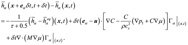 (2)
(2)
In the above equations,  and
and  are the particle distribution functions,
  is the a-direction microscopic particle velocity,
  is the time step,
  is the dimensionless relaxation time,
  is the macroscopic velocity,
  is the macroscopic density, and
  is the constant speed of the sound in D2Q9 model, see [26] . C is the composition of the heavy component,
  is the chemical potential,
  is the hydrodynamic pressure, and
  is the constant mobility.
  and
and  are the modified equilibrium distribution functions and defined by the following equations:
 (3)
(3)
 (4)
(4)
Considering  as the weighting factor in the D2Q9 model,
  and
and , the original equilibrium functions, are given by:
 (5)
(5)
 (6)
(6)
where
 (7)
(7)
Based on [17] , the mixing energy density for an isothermal system can be derived:
 (8)
(8)
where  is the gradient parameter and
 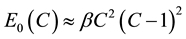 is the bulk energy.
  is a constant.
The classical part of the chemical potential,  , is related to the bulk energy by its derivative with respect to C, namely
 . Finally, when the mixing energy is minimized, the equilibrium profile is obtained.
 (9)
(9)
The composition, velocity, and hydrodynamic pressure can be computed by the following equations:
 (10)
(10)
 (11)
(11)
 (12)
(12)
Above equations are derived by taking the zeroth and first moments of the modified particle distribution functions. As seen from Equation (9), the equilibrium chemical potential is a function of the composition C, hence calculation of C by using the Equation (10) leads to a nonlinear iterative procedure. In this study we use the value of  from the previous time step in Equation (10). According to the appendix of [27] , this substitution still yields a second order accurate explicit scheme in time.
The Density and dimensionless relaxation time are computed from the following equations:
 (13)
(13)
 (14)
(14)
where  and
and  denote the bulk density and dimensionless relaxation time of the component i, respectively. Based on [18] the kinematic viscosity is then given by
 .
.
For a circular bubble with radius R, we use following equation as the interface profile at equilibrium:
 (15)
(15)
where z is the distance from the center of the bubble and D is the numerical interface thickness. Having D and , the gradient parameter
  and the coefficient of the surface tension
 , can be computed:
 (16)
(16)
 (17)
(17)
Ultimately, the total pressure, P, can be computed using the summation of the hydrodynamic pressure , the
, the
thermodynamic pressure , and pressure due to the curvature
 , see [28] .
At the last part of this section, we introduce the discretized forms of the first and second derivatives used in the current research. In the case of D2Q9 model, by considering  as a macroscopic variable, such as C, the first and second derivatives are discretized as follows
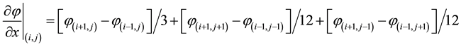 (18)
(18)
 (19)
(19)
 (20)
(20)
in which i and j are grid indices in the x and y direction, respectively. An almost thorough discussion of the above discretization schemes is provided in [18] .
2.2. Boundary Conditions
Before beginning the main discussion about the boundary conditions, it is worth to mention that in the present study by using the lattice links we model the smooth curved wall as a series of stair steps. Although this model results in geometric discontinuities and affects the computational accuracy, employing the LBM formula becomes straightforward on the wall boundary nodes.
By utilizing D2Q9 model and considering foregoing discretized forms of the first and second derivatives, naturally, the evaluation of the  and
and  at a typical node requires values of
  at all of its eight neighbors. For visual representation, two fluid and wall boundary nodes within their neighbors are shown in Figure 1. From this figure it can be seen that calculation of the
  and
and  at a boundary node depends on the values of
  at its solid neighbors. Therefore the values of
  at such solid nodes adjacent to boundary nodes should be updated at every iteration of the solution. In a recent research by Lee and Liu [28] , by assuming the straight wall as a mirror, the profile of
  at the solid nodes takes the mirror image of
  at the counterpart fluid nodes. They developed the claim that this scheme imposes no flux condition and prevents unphysical mass and momentum fluxes through the wall boundary. Although implementation of this approach is quite simple for straight wall boundary, it involves a detailed investigation for the curved one. The succeeding parts of this section are concerned with the modification of the mentioned approach for the curved wall boundary.
Following technique is quite practical for all kinds of boundary geometries. In the current study we consider a vertical right-orientated 90˚ bend as a case with curved wall boundary. The modification process can be divided into two main steps:
・ Step 1: First, the smooth curved wall is modeled by the lattice links and the arrangement of the boundary nodes is recognized. Based on the kind of neighbors (fluid, boundary, and solid), the type of all wall boundary nodes and tangent lines at each one are identified. For each type the lattice link perpendicular to the tangent line at the specified boundary node is considered. Now by assuming the tangent line as a mirror, the value of  at the solid node laid on the mentioned lattice link can be updated by the value of
  at the counterpart fluid node. All types of the wall boundary nodes appeared in the utilized 90˚ bend are shown in Figure 2, first four types appear in the bottom and right wall and last four ones appear in the top and left wall of the bend. In Figure 2, using the macroscopic variables of the fluid nodes marked with “F”, the macroscopic variables of the solid nodes marked with “S” are updated.
In some especial cases, one solid node can be updated by two fluid nodes. In such cases the solid node takes the average values of the two fluid nodes. Existence of such especial cases only depends on the arrangement of the boundary nodes. One may use a simple algorithm to search these cases. Such cases for the 90° bend are illustrated in Figure 3. The solid nodes marked with “S” takes the average values of the two fluid nodes marked with “F”.
・ Step 2: As noted earlier, the values of  at solid nodes adjacent to boundary nodes should be updated at every iteration of the solution. By completion of the first step, high percent of such solid nodes is recognized

Figure 1. Typical fluid and wall boundary nodes within their neighbors marked with “N”. “F” and “B” denote fluid and wall boundary nodes, respectively.

Figure 2. Illustration of all types of the boundary nodes in a vertical right-orientated 90˚ bend. In types 3, 4, 7, and 8 the tangent line coincides with the boundary line.
and by implementing the preceding scheme their macroscopic variables are updated. As is clear the arrangement of the boundary nodes merely depends on the line equation of the smooth curved wall. Accordingly based on this equation there may exist some state where the macroscopic variables of a solid node appeared in calculations remain constant during the solution. To solve this problem we use the average value of the two nearest solid neighbors updated in the first step. To find such states one may use an algorithm to check all solid nodes adjacent to boundary nodes and flag the ones which are not updated at the first step. Applying same algorithm for the specified 90˚ bend, all explained states are depicted in Figure 4. In this figure the macroscopic variables of solid nodes marked with “S” take the average values of the two nearest solid neighbors marked with “X”.
A closer look at the above two-step scheme indicates that all macroscopic variables of solid nodes adjacent to boundary nodes are updated during the solution. So far, all the effort in the previous treatment of the boundary conditions is to impose no flux condition at wall boundary nodes by updating the required macroscopic variables of the solid ones.
To accomplish prior description it is also worth noting that as an alternative method one may use first order modification at wall boundary. By considering a virtual boundary in the middle between lattice nodes, the values of boundary nodes can be directly updated by the values of counterpart fluid ones. In order to employ this method for the specified 90˚ bend, in Figure 2 the macroscopic variables of the boundary nodes marked with “B” should be updated by the variables of the fluid nodes marked with “F”.
Reviewing Equations (10), (11), and (12), it is obvious that distribution functions play a great role in the evaluation of the macroscopic variables. So we draw our attention to distribution functions at the wall boundary nodes. In the present study to obtain unknown particle distribution functions at such nodes we use familiar bounce-back scheme. It is crucial to note that this scheme is not limited to particle distribution functions stream-

Figure 3. Illustration of all cases where a solid node marked with “S” can be modified by two fluid nodes marked with “F”.

Figure 4. Illustration of all states where a solid node mark with “S” appears in the calculations with initial constant variables.
ing from boundary nodes to the fluid ones. Figure 5 gives an example of unknown particle distribution functions which should be modified to get accurate boundary conditions, e.g., zero velocity at the wall boundary nodes. To clarify above explanation, initially we employ streaming-collision step for all fluid and boundary nodes and afterward unknown particle distribution functions at boundary nodes are modified by applying simple bounce-back scheme. Although further study of this issue is still required, the proposed technique leads to quite acceptable results.
Lastly, the unknown  at the inlet and outlet of the channel is computed by using the scheme proposed by Zou and He [29] . Moreover, a second order extrapolation is used to compute the unknown
 ,
,  , and
, and  at these nodes. It is expected that the modified boundary condition can be readily extended to 3-D flow problems involving curved geometries.
2.3. Deformation Criterion
So far, a large body of literature has been devoted to the bubble and drop deformation under different conditions. However, there is no comprehensive criterion to describe the rate of the deformation quantitatively. Recently Amaya-Bower and Lee [23] have used the length L and the width W of the bubble to create a measure ofthe deformation, defined as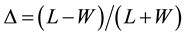 . Obviously this measure is only applicable in straight ducts. In this paper, to introduce a generalized criterion the variance of the lattice nodes constructing the bubble’s area with
respect to the centroid of the bubble is calculated at every iteration by , where
  is the dis-
tance between the node i and the centroid, and N is the number of the nodes constructing the bubble.  is
is
normalized by the polar radius of gyration of the initial circular bubble,  , where
  is the polar area moment of inertia, A is the area, and d is the diameter of the initial circular bubble. Clearly, more deviation from the initial circular shape leads to a higher value of
 . As a detailed analysis, one may calculate the
variance with respect to the x and y axes passed through the centroid of the bubble area, namely
 and
and , where
  and
and  are the distance between the node i and the x and y centroidal axes.
 and
and  can be normalized by the x-axis or y-axis radius of gyration of the initial circular bubble,
 . As a matter of fact,
  is a measure of the bubble extension along the y axis. However,
  provides a scale to determine the bubble deformation parallel to the x axis. In addition, to compare the deforma-

Figure 5. A typical state where the distribution functions never become modified in the directions depicted with the filled thick arrows.
tion rate in general one can use .
.
To the authors’ best knowledge, proposed criteria never have been used in the available literature that addresses the issue of drop or bubble deformation. One of the big advantages of above novel criteria is that they are practical in all kind of domain geometries and can be readily extended to 3-D simulations.
3. Validation
In order to validate the numerical method a common test in two phase flow simulations, the stationary bubble test, is conducted. As discussed in [18] generally the discretization error decreases with interface thickness D. Thus a larger D leads to a better agreement with the analytic prediction. Moreover, as long as the value of the numerical interface thickness D is high enough to use an isotropic discretization, D has very little to no effect on the shape of the bubble, see [22] . In another paper by Lee [19] the effects of mobility M on the parasitic currents were investigated. It was shown that higher values of M accelerate the rate of the convergence toward the equilibrium state. Accordingly we set  and
and  in all ensuing simulations. To implement validation test, remaining parameters are designated as follows:
  for both components,
  , and
, and . The index “1” and “2” correspond to the fluid surrounding the bubble and the fluid inside the bubble, respectively. By utilizing D2Q9 model, two dimensional bubbles with different radii are generated at the center of a
  computational domain with wall boundaries. The simulation is performed for three different values of the interface tension,
  , and the pressure difference inside and outside the bubble is measured at a
dimensionless time , where
  and
and . In the preceding equations R is the ra-
dius of the bubble at equilibrium and . So far we have numerically determined the pressure difference through the interface.
According to the Laplace law, one can analytically compute the pressure difference across the interface of a two dimensional bubble by using the following equation:

where  and
and  are the pressures inside and outside the bubble, respectively.
As depicted in Figure 6 it is clear that numerical results (the squares) are in a good agreement with the analytical solution obtained from Laplace law (the straight lines). As a result the surface tension is successfully modeled.

Figure 6. Verification of the Laplace law for  computational domain with wall boundaries.
 ,
,  and
and .
.
4. Numerical Results
4.1. Parameter Setup
To gauge the capabilities of the utilized wall boundary condition, proposed in this paper, a series of 2-D analysis will be carried out in the following sections. For this purpose, a straight duct and a vertical right-orientated 90˚ bend with constant width is utilized. In the absence of the gravity, uniform velocity and fully-developed condition are applied as boundary conditions at the inlet and outlet of the channels, respectively. To characterize two phase flow with mentioned boundary conditions, first, we introduce the parameters contributing to the deformation of a single bubble in a 2-D straight duct. There are twelve independent dimensional quantities: the uniform inlet velocity , the densities
  and
and , the viscosities
  and
and , the coefficient of the surface tension σ, the width of the channel W, the length of the channel L, the coordinates of the center of the initial bubble
 , the diameter of the initial bubble d, and the simulation time t. The geometric configuration of the problem is illustrated in Figure 7(a). According to the Π-theorem of dimensional analysis, nine independent non-
dimensional numbers can be formed to completely describe the problem. These parameters are ,
,  ,
,  ,
,  , density ratio
 , viscosity ratio
 , the nondimensional time
 , the Reynolds, and the Weber number.


Reviewing the literature, different parameters are used in the definition of the Reynolds and the Weber numbers. In the current study we use the inlet velocity , the width of the channel W, and the properties of the continuous phase,
  and
and , as the characteristic quantities.
As a better study of the deformation of a single bubble in the specified 90˚ bend two straight channels with length of  and
and  are utilized before and after the bend respectively. The geometric configuration is demon
strated in Figure 7(b). To characterize two phase flow in such geometry, by using  and
and  instead of
 , all above dimensionless groups are involved.

Figure 7. Configuration of the utilized (a) straight duct and (b) vertical right- orientated 90˚ bend with the initial circular bubble placed in the channel.
4.2. Grid Resolution Dependence
By considering the straight duct a grid resolution analysis is carried out. We use four different grid sizes,
 ,
,  ,
,  , and
, and . The evaluation is performed for constant values of
 ,
,  ,
,  ,
,  ,
,  ,
,  ,
,  ,
,  , and
, and . In addition, the values of
 , and
, and  are held fixed and the domain dimensions are normalized with the width of
the channel W in all subsequent simulations. Initially, by considering  at all fluid nodes inside the channel, single-component flow is modeled. Afterwards, at
  when a steady state is completely attained, a circular bubble is generated and the solution is continued. Figure 8 outlines the shapes of the bubbles for above grid resolutions at
 . It is evident that the general shape of the bubble for different cases remains constant. It is expected that by increasing the grid resolution bubbles become closer and overlap each other.
4.3. Length of the Channel Dependence
In the present work we use uniform velocity and fully-developed condition at the inlet and outlet of the channels, respectively. As one may speculate at this point, changing the length of the channel does not affect the shape of the bubbles. Actually, it is expected that the general flow pattern containing velocity remains constant as the length of the channel varies.
To assess this claim in the straight duct, the simulation is carried out for three different values of , and constant values of
 ,
,  ,
,  ,
,  ,
,  ,
,  ,
,  , and
, and .
.
Like before, first a steady state is completely attained and then at  a circular bubble is generated. Snapshots of the bubbles at
  are depicted in Figure 9. Obviously the bubbles are almost overlapping each
other and the effect of the channel’s length can be ignored. Accepting the fact that  has no effect on the de-
formation of the bubble, in the 90˚ bend  and
and  are held fixed.
Considering the results of two previous sections, to provide reasonable accuracy and avoid high computational cost, in all following simulations the width of the channel is set to be 64 lattice nodes. Furthermore, from now
on we set ,
,  , and
, and , where
  and
and  are the inner and outer radius of the
bend, see Figure 7(b). Correspondingly the grid sizes for the straight duct and 90˚ bend are 64 × 512 and 256 ×
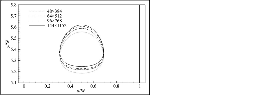
Figure 8. Effect of the grid resolution on the shape of the bubble passing through the straight duct at t* = 6.

Figure 9. Effect of the channel’s length on the shape of the bubble passing through the straight duct at t* = 6.
256, respectively.
4.4. Pressure Difference and Mass Flow Rate Ratio
Before exploring effects of the dimensionless numbers on the deformation of a single bubble, we address the pressure drop and mass flow rate ratio along the specified 90˚ bend. For this we use following parameters: ,
,  ,
,  ,
,  for both components,
 . At
. At , when a steady state of the single-component flow is fully obtained, a circular bubble with
  is generated at
 . The simulation is continued up to
  to investigate the influence of the bubble motion on the other variables. Velocity vectors immediately after constructing the bubble can be found in Figure 10. As can be seen generating the bubble brings about disturbance in the velocity field which are almost vanished at
 . For
. For
more inspection Figure 11 presents the mass flow rate ratio  and dimensionless total pressure difference
 , where
  and P is the total pressure. The provided graphs indicate that the fluctuations
occurred at  are damped rapidly and the velocity and pressure fields get back their earlier states.
Also Figure 11 implies that  remains constant which is equal to the pressure drop along the channel. In addition, the mass flow rate ratio converges to one, therefore there is no mass flux across the curved wall boundary. To accomplish a thorough check, streamlines and dimensionless total pressure contours for the single- component flow at the steady state is illustrated in Figure 12. Consequently the modified boundary condition correctly establishes the velocity and pressure fields.
From now on, first, the steady state of the single-component flow is modeled and then the bubble is generated at . Moreover, in all succeeding simulations same stated boundary conditions are applied to the straight duct and 90˚ bend outlined before.
4.5. Weber Number Effect
Generally speaking, one may consider the Weber number, the ratio between the inertia and the surface tension, as the most important dimensionless number in the deformation of a single bubble under the zero gravity condition. To investigate the Weber number effect on the deformation of a bubble, other parameters are held constant:
 ,
,  ,
,  ,
,  ,
,  , and
, and . By varying
  three cases are evaluated:


Figure 10. Velocity vectors near the generated bubble at t* = 3.00025 up to t* = 3.15. Initial disturbances are completely vanished at t* = 3.15.

Figure 11. (a) Total nondimensional pressure difference,  , and (b) mass flow rate ratio,
  , for the 90˚ bend. at t* = 3, the bubble is generated.
 . Results of the simulations for the straight duct and 90˚ bend are given in Figure 13 and Figure 14, respectively. As shown in Figure 13, at lowest Weber number,
  , the bubble tends to preserve its initial circular shape. In this case, high surface tension force does not allow the bubble to deform and stretch to the

Figure 12. Streamlines and nondimensional total pressure contours for the single-component flow at the steady state for the 90˚ bend.

Figure 13. Effect of the Weber number on the deformation of the bubble passing through the straight duct. ,
,  ,
,  ,
,  ,
,  , and
, and .
.
high-speed region of the channel. Hence, the bubble has a kind of a rigid body motion with the lowest speed of its particles. As illustrated in Figure 14, an almost same process is occurred at the bend, but this time, geometric configuration of the wall boundary leads to a more sensible deformation.
By increase of the Weber number to , the bubble stretches to the middle of the channel. As seen in Figure 13, this procedure just happens at the beginning stages and the bubble takes its final shape rapidly, the oblique circular cap with an almost straight line at the base of it. This oblique state will be vanished and turn into a direct one if we continue the simulation. In the 90˚ bend, in addition to the changes of velocity magnitude versus the width of the channel, the direction of the velocity vector varies continuously along the channel. As a result, the bubble maintains its deformed shape for more time, see Figure 14.
With further increase of the Weber number to , the inertial force becomes dominant and the bubble

Figure 14. Effect of the Weber number on the deformation of the bubble passing through the 90˚ bend. ,
,  ,
,  ,
,  ,
,  , and
, and .
.
deforms easily. Therefore the bubble sustains its stretched form along the channel to access to the region with the highest velocity, the middle of the channel, as a result the bubble can travel more distance. The final shape is almost similar to , but the bubble is more prolate, see Figure 13. As the Weber number increases, the bubble becomes more stretched and slender. In the straight channel at the end of the 90˚ bend, when the bubble starts to concentrate and take its final shape, it is possible that some parts of the bubble separate from the main part.
This phenomenon is shown in Figure 14. As well as the Weber number, by changing the other dimensionless numbers, this state can be intensified or weakened.
To analyze above discussion quantitatively ,
,  , and
, and  are plotted against
  for the 90˚ bend in Figure 15. Clearly the analysis indicates that the case with
  has the highest magnitude of the
  in all three diagrams. On the other hand for the case with
  the value of
  just fluctuates around one which
signifies that when the surface tension force is comparable with the inertia force, bubble tends to preserve its in- itial circular shape. Now we explain the pattern of the bubble deformation for the case with . First, the
bubble becomes stretched and inclines toward the middle of the initial straight channel, consequently  and
and

Figure 15. (a) , (b)
, (b) , and (c)
  against
  for the 90˚ bend. Effect of the Weber number on the deformation of the bubble passing through the 90˚ bend.
 ,
,  ,
,  ,
,  ,
,  , and
, and .
.
 increase though
  remains almost constant. At this occasion stretching and obliqueness act in the opposite direction for
 . The bubble takes the maximum value of
  at
at , at this stage bubble experiences the main rotation through the bend and reorients to horizontal direction. As time goes on the minimum value of
  and the maximum values of
  and
and  take place at
 . From this and by reviewing Figure 14 we
can deduce that the peak of the deformation rate occurs at the end of the bend, just at the beginning of the horizontal straight channel. With further progress in time as elongated bubble inclines toward the middle of the horizontal channel, it starts to concentrate and take its final shape. Accordingly we are witness to the reduction in
the deformation rate which are visible in the  and
and . Due to the separation occurred at
  there is another maximum at the value of
  for the case with
 . In fact tiny separated part quickly takes its final shape and diminishes the deformation rate.
Interestingly by reducing the amplitude, bubble deformation of the two other cases follows the same pattern as the discussed one, . However, it should be noted that the extremums of deformation rate for the different cases do not take place at a same time or location. Actually bubbles with lower level of the Weber number encounter extremums sooner than the others. In view of all that has been mentioned so far, one may suppose that heightening the Weber number leads to a delay in the reaction of the bubble to the continuous phase circumstances, e.g. velocity vectors.
In the current section we provided all three introduced deformation criteria to comprehend the relationships between them. Hereafter in the following sections to prevent repetitive analysis we just investigate the diagram
of .
.
4.6. Initial Bubble’s Coordinate Effect
When the surface tension force becomes negligible, the velocity dissimilarity between the particles constructing the bubble plays a significant role in the deformation. In this state, if the velocity magnitude difference between the particles heightens, the bubble becomes stretched. This phenomenon can be intensified or weakened by the velocity direction distinction. To probe this issue, we repeat the simulation for the straight duct by considering
constant values of ,
,  ,
,  ,
,  ,
,  ,
, . The simulation is carried out for
  and
and . One can easily observe the effect of the velocity magnitude difference on the deformation of the bubble in Figure 16. At
 , a high difference in the velocity magnitude of the left and
right side of the initial bubble leads to an intense deformation. By approaching to the middle of the channel, the particles of the bubble take more similar velocities and the bubble loses its stretched shape. On the other hand, at
 , the bubble takes an almost steady shape and never experiences the stretched form.
To determine the influence of the direction of the velocity vector, the same simulation is performed in the 90˚
bend for  and
and . In Figure 17, where
 , the magnitude and the direction of
the velocity vector act in the same way and enhances the deformation, accordingly, the bubble stretches along the channel. On the contrary, at , the magnitude and the direction of the velocity vector diminish
each other’s influences and the bubble encounters a low rate of deformation.
We can now proceed analogously to the previous section.  is plotted against
  for the 90˚ bend in Figure 18. We can see that at the beginning of the simulation, as long as bubbles are moving through the vertical channel, both test cases have almost same deformation pattern. At
  when bubbles reach to the bend, the
diagrams definitely follow two different trends. At this time the case with  loses its stretch form
and undergoes a low rate of deformation. In fact at this stage velocity vectors orientation counteracts the effect
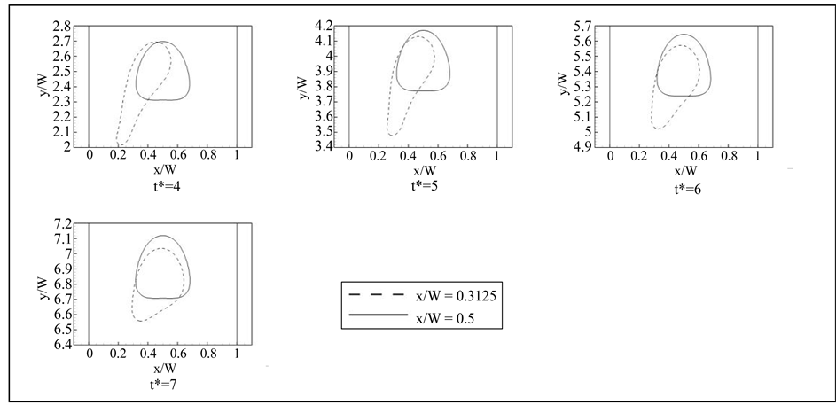
Figure 16. Effect of the initial bubble’s x-coordinate on the deformation of the bubble passing through the straight duct. ,
,  ,
,  ,
,  ,
,  ,
, .
.

Figure 17. Effect of the initial bubble’s x-coordinate on the deformation of the bubble passing through the 90˚ bend. ,
,  ,
,  ,
,  ,
,  ,
, .
.

Figure 18.  against
  for the 90˚ bend. Effect of the initial bubble’s x-coordinate on the deformation of the bubble passing through the 90˚ bend.
 ,
,  ,
,  ,
,  ,
,  ,
, .
.
of the velocity magnitude dissimilarity. At  as bubble approaches to the end of the bend, minimum
rate of deformation occurs. From now on there is a gradual rise in the value of  which is related to the bubble inclination toward the middle of the horizontal channel. In contrast, the case with
  precisely
demonstrates opposite manner, bubble becomes entirely extended throughout the bend and at  the highest level of extension appears.
Although 3-D studies are still required for a general conclusion, the data gathered in this section suggests that to expand the interface between two phases, one can rationally utilize curved pipes. Accordingly, by using a vertical right-orientated 90˚ bend, the dispersed phase should be injected from the left upright wall. This can be useful in different areas; for instance it is expected that increased interface between two phases leads to a higher mixing quality of two miscible phases and a better heat transfer efficiency. Inverse process can be implemented to minimize the interface as well.
Clearly, by considering the fully-developed condition before generating the bubble, one can easily perceive
that  has no effect on the deformation in the straight duct. Certainly the bubble should generate far enough
from the inlet of the channel. In the 90˚ bend, the influence of the  can be modeled in an altered way, in
other words, we can use another initial shape instead of the circular one with a different value of . For this
reason, the effect of the  is not studied in the current survey.
4.7. Bubble’s Diameter Effect
As mentioned before, when the Weber number is high enough, velocity field plays a key role in the deformation. By increasing the bubble’s diameter, the influence of the velocity field enhances. Furthermore, the viscous effect created by the wall boundary becomes more significant in the behavior of the bubble. To recognize the bubble’s
diameter dependence, the simulation is executed for three cases of , namely
 . The other pertinent dimensionless numbers are held fixed:
 ,
,  ,
,  ,
,  ,
,  , and
, and . It is apparent from Figure 19 that the smaller bubbles almost maintain their general forms throughout the trajectory in the straight duct. For the case with
  the shape remains egg-like with rounded top and bottom, albeit the case with
  takes a cap shape at top and a flattened base with a trivial dimple. The viscous effect imposed by the wall boundary becomes more discernible for the largest bubble with
 , the bub-
ble stretches at its sides and the dimple at the base becomes deeper. It seems that more continuous phase is trapped at such dimple as time passes. To assess this hypothesis we continue simulation. Figure 20 shows bub-
ble configuration for the case with  at
at . Surprisingly trailing parts at two sides of the bubble
detached from the leading part. We suppose that by changing the other parameters especially the Weber number one can accelerate or slow down the mentioned detachment. Further study of this issue would be of interest.
Overall the same procedure is happened in the 90˚ bend, see Figure 21. A closer look at the presented snapshots manifests the fact that such noted deep dimple never exists for the largest bubble in the 90˚ bend. To address this phenomenon we have to review the results of the previous section. Actually the part of the bubble rotating at a smaller radius rapidly coalesces though the portion at a distant radius sustains its deformed shape.
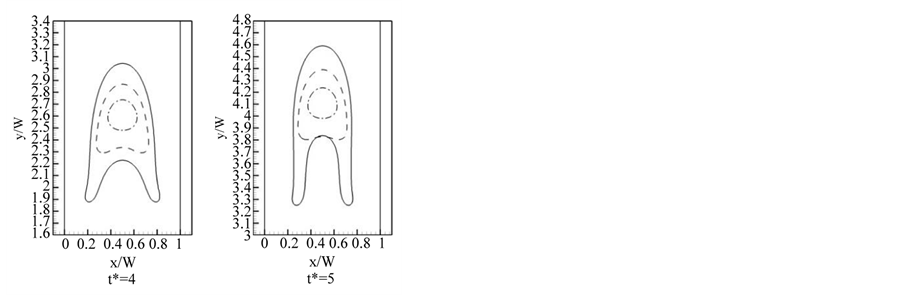

Figure 19. Effect of the bubble’s diameter on the deformation of the bubble passing through the straight duct. ,
,  ,
,  ,
,  ,
,  , and
, and .
.

Figure 20. Bubble configuration in the straight duct for the case with  at
at ,
,  ,
,  ,
,  ,
,  ,
,  , and
, and .
.
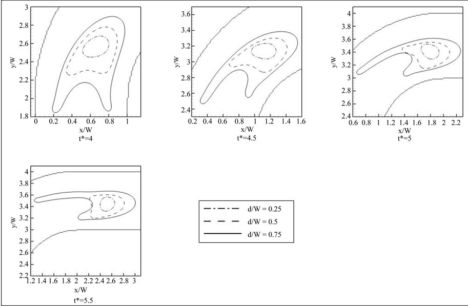
Figure 21. Effect of the bubble’s diameter on the deformation of the bubble passing through the 90˚ bend. ,
,  ,
,  ,
,  ,
,  , and
, and .
.
Plainly it is expected that larger value of  leads to a higher rate of deformation. Figure 22 illustrates
against  for the 90˚ bend. Despite the fact that there are extremums in the diagrams of the two cases with smaller diameter, the amplitude of the oscillations remains at low level. One can easily understand that there is a major difference between the deformation pattern of the largest bubble and the two other test cases. Strictly speaking the two cases with smaller diameter experience the maximum rate of deformation as moving through
the bend. On the other hand, as explained before, the symmetry of the bubble for the case with  decreases throughout the bend. Therefore it is predicable that the maximum rate of deformation takes place at the end of the bend. Zero slope of
  for the case with
  at
at  is a convincing evidence for the
foregoing claim.
4.8. Density Ratio Effect
The influence of the density ratio, defined by , is evaluated by comparing the bubble treatment of three different cases. Changing the value of
 , the test cases have density ratios of
 . Like preceding sections, first we set all other parameters:
 ,
,  ,
,  ,
,  , and
, and . To capture more

Figure 22. Effect of the bubble’s diameter on the deformation of the bubble passing through the 90˚ bend. ,
,  ,
,  ,
,  ,
,  , and
, and .
.
sensible deformation we intentionally create the initial bubble near the left wall, namely . In this
way the segments of the bubble located near the central line get moving faster, as a result, more noticeable deformation takes place. Simulated results for the straight duct are shown in Figure 23. As one can observe from the figure, change in the density ratio has a small effect on the layout of the interface. Looking closely at the position of the bubbles, it seems that the cases with lower density ratio reach smaller distances in the same amount of time. To explain these results, first, it should be remembered that the main cause of fluid flow along the channel is the constant pressure difference imposed by the utilized boundary conditions. One may interpret this situation as a constant force field along the channel. An important issue that should be noted here is that the density of the continuous phase remains invariant for above three test cases. Therefore by considering constant volume for the bubble as density ratio decreases, the density and mass of the fluid inside the bubble increase. Clearly the bubble with higher mass is thrust with smaller value of acceleration existed due to the constant force field, thus the smaller amount of the displacement is expected. In addition by varying the density ratio there is not any extra force exerting on the interface, as a result, the shape of the bubble is left unchanged for all test cases. The findings of the current study are consistent with those of [22] and [30] where the effect of density ratio on terminal velocity and shape of a bubble rising in a viscous liquid is well investigated. It is reported that effect of density ratio is more discernible in terminal velocity than in final shape. Although in these works the bubble rises due to gravitational force, it provides a good confirmation for the results obtained in this section.
Repeating the simulation for the 90˚ bend same results are obtained, in other words, there is a same deformation pattern with a slight difference in the positions of the bubbles, see Figure 24. As it was predictable, by approaching to the half of the bend, the case with the highest density ratio inclines to the wall boundary with smaller radius more than the others. A possible explanation for this is the well-known centrifugal force which
can be intensified by density ratio.  versus
  for the 90˚ bend is shown in Figure 25. There are some differences in the value of
  for foregoing test cases. We suppose that the major part of such distinction is re-
lated to the numerical inaccuracy in determination of the interface periphery and of course the lack of adequate

Figure 23. Effect of the density ratio on the deformation of the bubble passing through the straight duct. ,
,  ,
,  ,
,  ,
,  , and
, and .
.

Figure 24. Effect of the density ratio on the deformation of the bubble passing through the 90˚ bend. ,
,  ,
,  ,
,  ,
,  , and
, and .
.
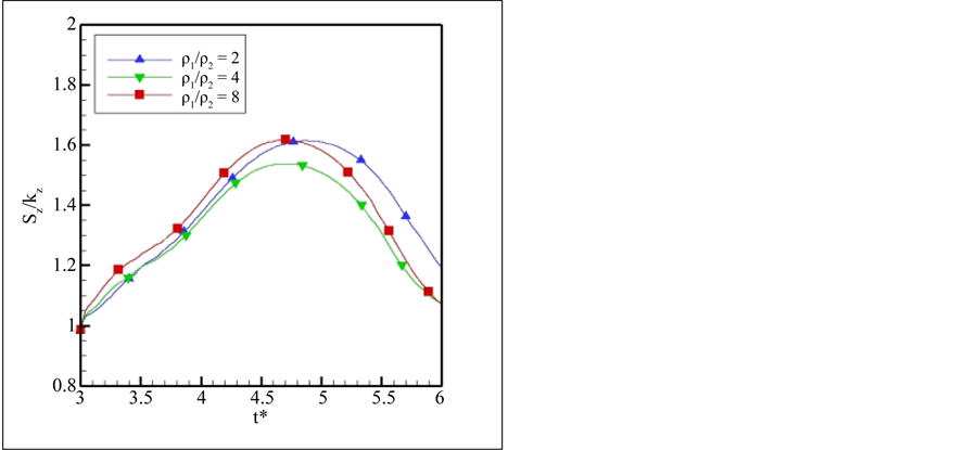
Figure 25.  against t* for the 90˚ bend. Effect of the den- sity ratio on the deformation of the bubble passing through the 90˚ bend.
 ,
,  ,
,  ,
,  ,
,  , and
, and .
.
mesh size. In general, presented graph further verifies the claim that effect of density ratio on the pattern of the deformation can be neglected.
4.9. Viscosity Ratio Effect
To study the effect of the viscosity ratio, defined by , all other parameters remain the same:
 ,
,  ,
,  ,
,  ,
,  , and
, and . Changing the value of
 , the test cases have viscosity ratios of
 . Results of the simulation for the straight duct and 90˚ bend are depicted in Figure 26
and Figure 27, respectively. A comparison of the bubble postures reveals that as the viscosity ratio increases, the interface becomes more immovable and the bubble behaves more like a rigid object. To analyze this kind of treatment, first, we recall that the constant pressure difference is the source momentum of the fluid flow. A critical feature that should be noticed at this point is that the viscosity of the continuous phase remains unchanged, therefore pressure drop along the channel is the same for all test cases. By increasing the viscosity ratio the friction between two phases becomes more significant and larger amount of energy dedicated to the bubble evolution dissipates at the interface. In consequence, the edges of the bubble become more prone to integrate which is corresponded to the lowest level of dissipation. Observing in detail, there is no clear correlation between the viscosity ratio and the position of the bubble.
As illustrated in Figure 28 there is a same pattern of deformation in the 90˚ bend, specifically, all three cases experience the maximum rate of deformation while passing through the bend. The most striking result emergingfrom the diagram is that the cases with higher viscosity ratio take their extremums in a shorter time. As discussed before absolutely inverse result takes place about the Weber number. These findings suggest that increase of any factor that enhances the rate of the deformation leads to a delay in the response of the bubble to the surrounding situations. In other words there is an inverse proportionality between the amplitude and frequency of the bubble deformation.

Figure 26. Effect of the viscosity ratio on the deformation of the bubble passing through the straight duct. ,
,  ,
,  ,
,  ,
,  , and
, and .
.
4.10. Reynolds Number Effect
The Reynolds number is defined as the ratio of the inertia to the viscous force. In the current study we use the properties of the continuous phase,  and
and , as the characteristic quantities, however, there are other alternatives in Reynolds number definition. To investigate the effect of Reynolds number on the deformation of the bubble, we change the value of
  to obtain following cases: Re = 4, 8, 16. Other pertinent dimensionless num-
bers are held constant: ,
,  ,
,  ,
,  ,
,  , and We = 8. Snapshots of the bubble
states at various dimensionless time in the straight duct and 90˚ bend are shown in Figure 29 and Figure 30, respectively. As could be seen from the figures, increase of the Reynolds number leads to a lower rate of deformation and makes the bubble motion slower. To analyze these results we reconsider the discussion of the previous sections where the pressure difference is recognized as the main reason of fluid flow. Obviously by decreasing the value of the , viscous dissipation at wall boundary and the pressure drop along the channel reduce. Same procedure occurs about the pressure difference at two ends of the bubble at a typical moment. Therefore there exists a smaller value of force exerting on the interface to drive the bubble through the channel. Considering a constant mass, all these factors result in a reduction in the acceleration and velocity of the bubble. Lastly the velocity magnitude dissimilarity between the particles constructing the bubble lessens, consequently, low rate of deformation takes place. Another possible explanation for the final result is that the Weber number
defined by the velocity of the centroid of the bubble,  , diminishes, accordingly, high surface tension does not allow the bubble to deform easily.
Figure 31 demonstrates  against
  for the 90˚ bend. The data of the diagram, while preliminary, sug-
gests that by increasing the Reynolds number lower rate of deformation is exhibited. In addition, the findings of this section confirm the fact that there is an inverse proportionality between the amplitude and frequency of the bubble deformation.

Figure 27. Effect of the viscosity ratio on the deformation of the bubble passing through the 90˚ bend. ,
,  ,
,  ,
,  ,
,  , and
, and .
.
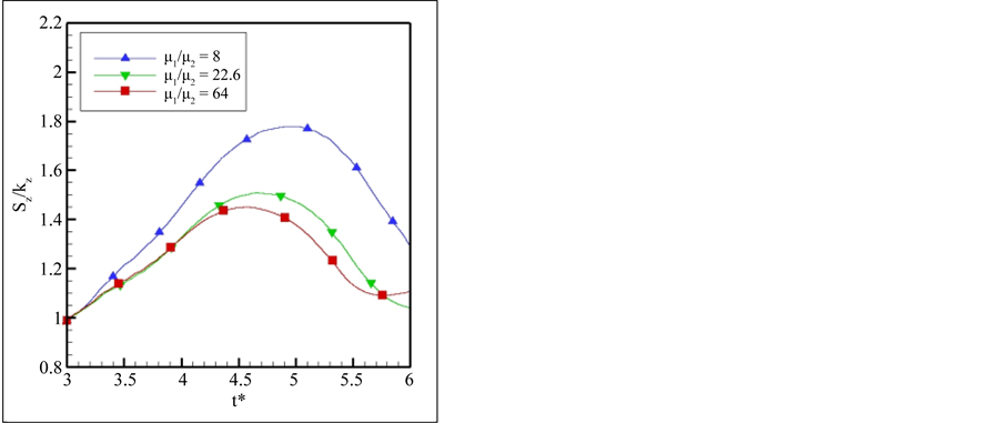
Figure 28.  against t* for the 90˚ bend. Effect of the viscosity ratio on the deformation of the bubble passing through the 90˚ bend.
 ,
,  ,
,  ,
,  ,
,  , and
, and .
.

Figure 29. Effect of the Reynolds number on the deformation of the bubble passing through the straight duct. ,
,  ,
,  ,
,  ,
,  , and
, and .
.

Figure 30. Effect of the Reynolds number on the deformation of the bubble passing through the 90˚ bend. ,
,  ,
,  ,
,  ,
,  , and
, and .
.

Figure 31.  against
  for the 90˚ bend. Effect of the Reynolds number on the deformation of the bubble passing through the 90˚ bend.
 ,
,  ,
,  ,
,  ,
,  , and
, and .
.
5. Summary
In this paper a thorough investigation of the deformation of a single bubble in a straight duct and a 90˚ bend in the absence of the gravity is presented. Extending the application of the LBM proposed by Lee [19] , an averaging scheme of boundary condition implementation has been presented to eliminate the mass and momentum
fluxes across the curved wall boundary. Calculating the pressure drop and mass flow rate ratio along the channel, it is shown that the proposed boundary condition establishes the velocity and pressure fields properly. A generalized benchmark, the nondimensional variance of the lattice nodes constructing the bubble area with respect to its centroid, has been utilized to find out the rate of the deformation.
Performing several 2-D simulations, it is seen that higher value of the Weber number leads to the increase of the deformation and the bubble stretches to the high-speed region of the channel more easily. Furthermore, geometric properties of the initial bubble, initial coordinates and the diameter, play a significant role in the fu- ture behavior of the bubble. Velocity dissimilarity between the particles of the bubble is determined as the main factor of the deformation for this case. Within the assumed range of the density ratio in the current study, analysis shows that it has a little effect on the shape of the bubble. Additionally, it is observed that as the Reynolds number or the viscosity ratio is decreased, higher rate of deformation is exhibited. Finally, as a general rule, it has been demonstrated that increase of any factor that enhances the rate of the deformation leads to a delay in the response of the bubble to the surrounding situations.
Cite this paper
Hamid Mohammad MirzaieDaryan,Mohammad HasanRahimian, (2015) Numerical Simulation of Single Bubble Deformation in Straight Duct and 90° Bend Using Lattice Boltzmann Method. Journal of Electronics Cooling and Thermal Control,05,89-118. doi: 10.4236/jectc.2015.54007
References
- 1. Grace, J.R. (1973) Shapes and Velocities of Bubbles Rising in Infinite Liquids. Transactions of the Institution of Chemical Engineers, 51, 116-120.
- 2. Bhaga, D. and Weber, M.E. (1981) Bubbles in Viscous Liquids: Shapes, Wakes and Velocities. Journal of Fluid Mechanics, 105, 61-85.
http://dx.doi.org/10.1017/S002211208100311X - 3. Fan, L. and Tsuchiya, K. (1990) Bubble Wake Dynamics in Liquids and Liquid-Solid Suspensions. Butterworth-Heinemann, Oxford.
- 4. Clift, R., Grace, J.R. and Weber, M.E. (1978) Bubbles, Drops and Particles. Academic Press, New York.
- 5. Prosperetti, A. and Tryggvason, G. (2007) Computational Methods for Multiphase Flow. Cambridge University Press, Cambridge.
- 6. Chen, L., Garimella, S.V., Reizes, J.A. and Leonardi, E. (1999) The Development of a Bubble Rising in a Viscous Liquid. Journal of Fluid Mechanics, 387, 61-96.
http://dx.doi.org/10.1017/S0022112099004449 - 7. van Sint Annaland, M., Deen, N.G. and Kuipers, J.A.M. (2005) Numerical Simulation of Gas Bubbles Behaviour Using a Three-Dimensional Volume of Fluid Method. Chemical Engineering Science, 60, 2999-3011.
http://dx.doi.org/10.1016/j.ces.2005.01.031 - 8. Ohta, M., Imura, T., Yoshida, Y. and Sussman, M. (2005) A Computational Study of the Effect of Initial Bubble Conditions on the Motion of a Gas Bubble Rising in Viscous Liquids. International Journal of Multiphase Flow, 31, 223-237.
http://dx.doi.org/10.1016/j.ijmultiphaseflow.2004.12.001 - 9. Bonometti, T. and Magnaudet, J. (2006) Transition from Spherical Cap to Toroidal Bubbles. Physics of Fluids, 18, Article ID: 052102.
http://dx.doi.org/10.1063/1.2196451 - 10. Feng, J. Q. (2007) A Spherical-Cap Bubble Moving at Terminal Velocity in a Viscous Liquid. Journal of Fluid Mechanics, 579, 347-371.
http://dx.doi.org/10.1017/S0022112007005319 - 11. Hua, J., Stene, J.F. and Lin, P. (2008) Numerical Simulation of 3D Bubbles Rising in Viscous Liquids Using a Front Tracking Method. Journal of Computational Physics, 227, 3358-3382.
http://dx.doi.org/10.1016/j.jcp.2007.12.002 - 12. Sukop M.C. and Thorne, D.T. (2006) Lattice Boltzmann Modeling: An Introduction for Geoscientists and Engineers. Springer, Berlin Heidelberg.
- 13. Yu, D., Mei, R., Luo, L.S. and Shyy, W. (2003) Viscous Flow Computations with the Method of Lattice Boltzmann Equation. Progress in Aerospace Sciences, 39, 329-367.
http://dx.doi.org/10.1016/S0376-0421(03)00003-4 - 14. Succi, S. (2001) The Lattice Boltzmann Equation: For Fluid Dynamics and Beyond. Oxford University Press, Oxford.
- 15. He, X., Chen, S. and Zhang, R. (1999) A Lattice Boltzmann Scheme for Incompressible Multiphase Flow and its Application in Simulation of Rayleigh-Taylor Instability. Journal of Computational Physics, 152, 642-663.
http://dx.doi.org/10.1006/jcph.1999.6257 - 16. He, X., Zhang, R., Chen, S. and Doolen, G.D. (1999) On the Three-Dimensional Rayleigh-Taylor Instability. Physics of Fluids, 11, 1143-1152.
http://dx.doi.org/10.1063/1.869984 - 17. Jacqmin, D. (1999) Calculation of Two-Phase Navier-Stokes Flows Using Phase-Field Modeling. Journal of Computational Physics, 155, 96-127.
http://dx.doi.org/10.1006/jcph.1999.6332 - 18. Lee, T. and Lin, C.L. (2005) A Stable Discretization of the Lattice Boltzmann Equation for Simulation of Incompressible Two-Phase Flows at High Density Ratio. Journal of Computational Physics, 206, 16-47.
http://dx.doi.org/10.1016/j.jcp.2004.12.001 - 19. Lee, T. (2009) Effects of Incompressibility on the Elimination of Parasitic Currents in the Lattice Boltzmann Equation Method for Binary Fluids. Computers & Mathematics with Applications, 58, 987-994.
http://dx.doi.org/10.1016/j.camwa.2009.02.017 - 20. Gupta, A. and Kumar, R. (2008) Lattice Boltzmann Simulation to Study Multiple Bubble Dynamics. International Journal of Heat and Mass Transfer, 51, 5192-5203.
http://dx.doi.org/10.1016/j.ijheatmasstransfer.2008.02.050 - 21. Fakhari, A. and Rahimian, M.H. (2009) Simulation of an Axisymmetric Rising Bubble by a Multiple Relaxation Time Lattice Boltzmann Method. International Journal of Modern Physics B, 23, 4907-4932.
http://dx.doi.org/10.1142/S0217979209053965 - 22. Amaya-Bower, L. and Lee, T. (2010) Single Bubble Rising Dynamics for Moderate Reynolds Number Using Lattice Boltzmann Method. Computers & Fluids, 39, 1191-1207.
http://dx.doi.org/10.1016/j.compfluid.2010.03.003 - 23. Amaya-Bower, L. and Lee, T. (2011) Numerical Simulation of Single Bubble Rising in Vertical and Inclined Square Channel Using Lattice Boltzmann Method. Chemical Engineering Science, 66, 935-952.
http://dx.doi.org/10.1016/j.ces.2010.11.043 - 24. Tölke, J., Freudiger, S. and Krafczyk, M. (2006) An Adaptive Scheme Using Hierarchical Grids for Lattice Boltzmann Multi-Phase Flow Simulations. Computers & Fluids, 35, 820-830.
http://dx.doi.org/10.1016/j.compfluid.2005.08.010 - 25. Yu, Z., Yang, H. and Fan, L.S. (2011) Numerical Simulation of Bubble Interactions Using an Adaptive Lattice Boltzmann Method. Chemical Engineering Science, 66, 3441-3451.
http://dx.doi.org/10.1016/j.ces.2011.01.019 - 26. Qian, Y.H. and Chen, S.Y. (2000) Dissipative and Dispersive Behaviors of Lattice-Based Models for Hydrodynamics. Physical Review E, 61, 2712.
http://dx.doi.org/10.1103/PhysRevE.61.2712 - 27. Lee, T., Lin, C.L. and Chen, L.D. (2006) A Lattice Boltzmann Algorithm for Calculation of the Laminar Jet Diffusion Flame. Journal of Computational Physics, 215, 133-152.
http://dx.doi.org/10.1016/j.jcp.2005.10.021 - 28. Lee, T. and Liu, L. (2010) Lattice Boltzmann Simulations of Micron-Scale Drop Impact on Dry Surfaces. Journal of Computational Physics, 229, 8045-8063.
http://dx.doi.org/10.1016/j.jcp.2010.07.007 - 29. Zou, Q. and He, X. (1997) On Pressure and Velocity Boundary Conditions for the Lattice Boltzmann BGK Model. Physics of Fluids, 9, 1591-1598.
http://dx.doi.org/10.1063/1.869307 - 30. Hua, J. and Lou, J. (2007) Numerical Simulation of Bubble Rising in Viscous Liquid. Journal of Computational Physics, 222, 769-795.
http://dx.doi.org/10.1016/j.jcp.2006.08.008