Theoretical Economics Letters
Vol.08 No.15(2018), Article ID:88635,16 pages
10.4236/tel.2018.815203
Effect of Confidence Shock on an Economy with a Shadow Banking System: Analysis Based on Dynamic Stochastic General Equilibrium Model
He Cong1, Yang Chen2
1Institute of Economics, School of Social Sciences, Tsinghua University, Beijing, China
2School of Economics, Peking University, Beijing, China

Copyright © 2018 by authors and Scientific Research Publishing Inc.
This work is licensed under the Creative Commons Attribution International License (CC BY 4.0).
http://creativecommons.org/licenses/by/4.0/


Received: October 18, 2018; Accepted: November 18, 2018; Published: November 21, 2018
ABSTRACT
We introduced a financial intermediary system including shadow banks into a New-Keynesian dynamic stochastic general equilibrium framework and analyzed the effect of confidence on the real economy. A model simulation indicated that confidence boosts growth and promotes consumption and investment in the real economy. The effects on the shadow banking system and traditional commercial banking system differed, thereby providing a new perspective for policy-making and economic structure model research.
Keywords:
Shadow Banking, Optimism, Dynamic Stochastic General Equilibrium Model, Confidence Shock

1. Introduction
The subprime mortgage crisis in the United States in 2007 evolved into the most serious international financial disaster since the Great Depression and changed the trend of global economic development. Ever since, demand in the global economy has been relatively weak and volatile, and the effects continue 10 years on.
The overall financial structure change, market failure, and excessive risky speculation were the internal causes of the crisis. In relation to these aspects, the shadow banking system had crucial influence. Shadow banking in the United States turns securitizations of poor liquidity into assets. Mortgage loans, credit card loans, and other liabilities are securitized and traded in the secondary market. Securities such as mortgage-backed securities and collateralized debt obligations are distributed to various financial institutions and held by the public, and shadow banks infiltrate every aspect of the financial system [1] . Although shadow banks are gradually replacing commercial banks to provide credit services, their current situation lacks supervision [2] . In 1982, the Garn-St. Germain Depository Institutions Act relaxed regulatory restrictions and facilitated large-scale expansion of mixed businesses operated by shadow banks. In September 2012, the total assets of shadow banks accounted for US$20.59 trillion, which was considerably higher than the US$17.51 trillion in assets of insurance companies and pension funds and the US$15.11 trillion of commercial banks [3] .
In contrast to commercial banks, the shadow banking system has no corresponding deposit insurance system or central bank support; therefore, it is highly sensitive to the effects of market sentiment. This is reflected by not only the large-scale expansion and development of shadow banking system during the economic boom but also the overall financial panic caused by bank runs in the shadow banking sector during the collapse of confidence.
This paper explores the effect of confidence on financial intermediaries, which helps to explain the logic behind the formation and growth of shadow banking.
The model that we set up has two key features. First, we assume homogeneity in the household sector and heterogeneity among banks and firms. Second, we modeled the confidence effect and applied it to investigate the influence of confidence on the shadow banking system, the overall financial environment and economic development channels. Diverse responses of different sectors help to identify the impact of confidence shock, and make it possible to shed light on the transmission channel of shadow banks under the influence of economic fluctuation.
The simulation results indicate the existence of channel slinking confidence with different financial intermediaries. We also proposed that shadow banking has a substitution effect on commercial banks in a prosperous economy.
The remainder of this paper is organized as follows. In Section 2, we describe our model, giving particular attention to the setup of optimism. In Section 3, the parameters and basis for the assignment are explained. The results are presented in Section 4 alongside analysis based on economic facts. Section 5 concludes this paper.
2. Related Literature
The definition of shadow banking was first put forward by PIMCO (Pacific Investment Management Company) executive director Paul McCulley at Federal Reserve’s Annual Meeting in 2008. It can broadly be described as “credit intermediation involving entities and activities outside the regular banking system” [4] .
From the start of the crisis there has been an explosion of literature about shadow banking. Most of the early literature focuses on the role of shadow banking in the crisis. Pozsar argued that the shadow banking system was a highly levered off-balance sheet vehicles, which was at the heart of the credit crisis [1] . Adrian and Shin analyzed the rise and impact of shadow banking from the perspective of securitization [2] . A comprehensive overview of the shadow banking system can be found in Pozsar, Adrian, Ashcraft, and Boesky [5] and Adrian and Aschcraft [6] .
Dynamic general equilibrium framework is widely used in the study of credit intermediaries and financial instability, which are closely related to the study of shadow banking. Bernanke, Gertler and Gilchrist pointed out the channels by which the financial market amplifies the impact market shocks [7] . This financial accelerator is also triggered by shadow banking sector, because shadow banks can also create credit. Christiano, Motto and Rostagno [8] built on the basic structure of Smets and Wouters [9] enlarged with Bernanke’s approach. Taking the activity of shadow banking into consideration, they found that liquidity constraints and shocks that alter the perception of market are the determinants of economic fluctuations. A simplified framework was developed by Verona, Martins and Drumond features over-optimism and over-leveraging in the course of the boom [10] . And a large number of literature studies the confidence effect, especially the banking panic and confidence collapse (see Diamond and Dybvig [11] , Gorton et al. [12] , Ferrante [13] ).
In summary, previous studies mainly focused on the financial instability and confidence effect on the whole economy. This paper combines these two important topics, investigate the channel through which confidence affects the shadow banking sector therefore changes the economic structure.
3. Model
This study modified the Verona’s model framework, which follows those of Christiano et al. [14] and Bernanke et al. [7] and includes the effect of confidence disturbance. We introduced financial friction, adjustment cost of investment, information asymmetry, and parallel financial intermediaries into a classic DSGE model.
In the model, each household is a monopolistic supplier of a differentiated labor service. The households earn wages and acquire dividends from ownership of firms, choosing consumption and savings. Monopolistic intermediate-goods firms employ labor from households and use capital services from entrepreneurs to produce intermediate products. The final-goods market is perfectly competitive, and final-goods firms combine intermediate goods to produce final goods. Final products are consumed by households and invested into capital production. Investments enter the hands of capital producers, who generate new capital through new investments and repurchases of depreciated capital products. Old capital repurchased by a capital producer can be converted one-to-one into new capital. New capital goods are to be sold to entrepreneurs.
An entrepreneur buys new capital from a capital producer at the end of period t, chooses the utilization rate in period t + 1, rents the capital to an intermediate-goods firm, and sells the depreciated capital to the capital producer at the end of period t + 1. Entrepreneurs are divided into high risk and low risk; this is the core setting of this model. High-risk entrepreneurs acquire loans from commercial banks, whereas low-risk entrepreneurs acquire loans from the shadow banking system.
3.1. Low-Risk Entrepreneurs and Shadow Banks
1) Low-risk entrepreneurs
In the model, a low-risk entrepreneur is denoted by L, whereas l represents low-risk entrepreneurs. The proportion of low-risk entrepreneurs among all entrepreneurs is . Each low-risk entrepreneur decides the capital utilization rate , scale of borrowing, and amount of capital purchased in each period. At the beginning of each period, low-risk entrepreneurs use the stock capital purchased at the end of the preceding period to generate capital services. That is, capital services for intermediate-goods production are . The cost of providing capital services increases with the utilization rate of capital. At the end of the process, the capital of a low-risk entrepreneur depreciates at rate . The entrepreneur sells the depreciated capital to a capital producer, repays the loan from the preceding period, acquires a loan for the next period, and purchases stock capital for the next period.
The liability is
where denotes the price of capital, denotes the liability of low-risk entrepreneur l, and is the net worth of low-risk entrepreneur l.
The utilization rate cost is
where denotes the real rental rate of capital service.
Considering optimal capital utilization, low-risk entrepreneurs follow this maximization principle:
where is the price level and denotes the loan rate of shadow banking system.
The first-order condition with respect to and is
,
where is the first derivative of the utilization cost function.
In each period, entrepreneur l’s equity is
Suppose that in each period, entrepreneurs exit the market with probability and transfer their assets to shareholders, namely households. Simultaneously, a new entrepreneur is born with probability and receives net worth from households.
Therefore, .
2) Shadow banks
Shadow banks have a certain bargaining power; therefore, entrepreneurs choose the optimal loan according to their interest rate cost when selecting a shadow bank. By contrast, shadow banks adjust their interest rates to maximize their own profits. Taking shadow bank z as an example; that is,
subject to .
In these equations, is the interest rate elasticity of the demand for funds.
Suppose .
Then, .
Shadow bank z should maximize its profits as
subject to
where is the base rate (i.e., the central bank’s target nominal interest rate).
The first-order condition is
.
According to the symmetric equilibrium condition, the following formula can be derived:
.
The profit of the shadow bank is .
To introduce the effects of optimism and confidence shock, we first assume , where the elasticity is constant.
The elasticity is affected by optimism, denoted as :
.
Here, indicates the overall feeling of optimism in the society. This value is higher than the steady-state optimism level because of the increase in net assets, which enhances the risk preference of operators and lowers interest rates; therefore, the whole economy enters a growth period or even a bubble period.
Under this assumption, a confidence shock can be expressed as
where is the shock to the overall economy, is the steady-state level of net worth, captures the degree of persistence in optimism, and is the sensitivity of optimism with respect to the deviation of the entrepreneur’s net worth.
3.2. High-Risk Entrepreneurs and Commercial Banks
1) High-risk entrepreneurs
The setting of high-risk entrepreneurs is essentially the same as that of low-risk entrepreneurs; H represents high-risk entrepreneurs and h represents a high-risk entrepreneur. The proportion of high-risk entrepreneurs among all entrepreneurs is . High-risk entrepreneurs must consider the utilization rate of capital, the cost of which is , and capital services acquire a real return rate of . The depreciation rate of capital is . The balance sheet is similar to that of low-risk entrepreneurs and can be expressed as .
In contrast to low-risk entrepreneurs, the level of capital stock of high-risk entrepreneurs is subject to a stochastic shock at each stage, following a
log-normal distribution: . Consequently, the stock capital of high-risk entrepreneur h is .
The return on capital service of high-risk entrepreneur h is
.
Because follows a log-normal distribution and all entrepreneurs are symmetrical, this formula can be rewritten as
Therefore, the optimal choice of high-risk entrepreneurs is to consider the capital utilization rate: .
The first-order condition is .
2) Commercial banks
When commercial banks make loan decisions, they know that high-risk entrepreneurs face risk shocks. When the risk shock faced by an entrepreneur is sufficiently high that the entrepreneur can only declare bankruptcy and return their net value to commercial banks, the bank bears some of the losses and pays a monitoring cost to retrieve the value. This assumption reflects the financial friction arising from asymmetric information between entrepreneurs and banks.
To control risk, the bank sets a risk threshold as a basis for the loan interest rate. Suppose is the gross interest rate on a loan; the threshold of risk is expressed as
.
According to the perfect-competition zero-profit condition,
Similar to low-risk entrepreneurs, in each period, the high-risk entrepreneurs exit with probability and transfer their assets to the shareholders, namely households. Simultaneously, a new entrepreneur is born with probability and acquires their net worth from households.
The process can be expressed as
.
.
3.3. Capital Producers
Capital producers are established according to the classic model’s setting. If capital producers are assumed to be perfectly competitive, old capital and new investment can be converted one-to-one into new capital, whereas investment has a certain adjustment cost:
The new assets generated by capital goods producers are
The maximization problem of capital producers is
The first-order condition is
The aggregate capital stock evolves according to
3.4. Final-Goods Firms and Intermediate-Goods Firms
1) Final-goods firms
The final-goods firms add up the intermediate goods to obtain the final output and sell part to the households for consumption and part to the capital producer as investment for production of capital goods.
The production function is
where , is the markup for the intermediate-goods firms.
The optimal choice for a final-goods firm is
2) Intermediate-goods firms
As monopolistic competitive enterprises, intermediate-goods firms have bargaining power. They employ labor provided by household at cost and rent the capital services of entrepreneurs to produce heterogeneous goods. In the case of a given output, the intermediate product operator minimizes the cost of production:
.
Thus, firm i’s optimal demand for capital and labor service must solve the following minimization problem:
subject to
where , denotes the capital share of production.
The first-order conditions with respect to and are
By combining these equations, we can derive the no-arbitrage condition:
Because all firms face the same input prices and have access to the same production technology, real marginal cost is identical across firms. By integrating the first-order condition and no-arbitrage condition into the cost function, we get
.
Intermediate-goods firms follow the assumption of Calvo [15] ; firms can adjust their price with probability . In addition, firms that cannot reset their price to the optimal level can change their price according to the changing inflation rate :
,
where is the steady-state level of inflation.
Based on the aforementioned assumptions, rational intermediate-goods firms optimize their profits through this operation:
.
Finally, we get
where
.
3.5. Households
The utility function of households is
where denotes consumption, is the amount of labor supplied, is the elasticity of the labor supplied, and is the preference parameter that affects the disutility of supplying labor.
The budget constraint of households is
where and are the interest rate of depositing in commercial banks and the return rate of shadow bank bonds, respectively; is the deposit in commercial banks; is the bond of the shadow banking system held by the household; represents the profit of intermediate-goods firms; and indicates the profit of the shadow banking sector.
The first-order condition can be calculated as follows:
.
According to these equations, , which means that at the equilibrium, households have no opportunity for arbitrage.
For the setting of the labor market, we introduce the hypothesis of labor heterogeneity to render the model more approximate to the real economy and improve simulation accuracy. Households can adjust their wage levels with probability . The aggregate labor demand is
The wage level is
.
Intermediate-goods firms make decisions based on the following formula:
.
The optimal choice of households with bargaining power in the pricing of labor is
subject to .
Households that cannot adjust their wages to the optimal level follow the dynamic process, expressed as
.
To facilitate representation and consider the application of symmetry, parts of this equation can be expressed as follows:
Finally, we obtain the following first-order conditions for maximization of household income:
.
3.6. Central Bank’s Monetary Policy
The central bank sets the short-term nominal interest rate following the Taylor rule.
Here, represents interest rate smoothing; and are the weights assigned to expected inflation and the output gap, respectively; is a white-noise monetary policy shock; and and are the steady-state values of inflation and output, respectively.
4. Calibration
To solve the steady-state solution more conveniently, the method and parameter settings of Christiano et al. [8] and Verona et al. [10] were consulted. We set the capital return rate ( ) of a high-risk entrepreneur as an exogenous variable with a value of 0.0504, in line with the value used by Christiano [8] . The weight of labor disutility was set as an endogenous variable; its value could be obtained by calculating the steady-state solution. The parameters in the model were calibrated and their references are shown in Table 1.
5. Results and Analysis
According to the model hypothesis and parameter assignment, we simulated the disturbance of confidence oscillation. The results are shown in the following diagrams, which show the responses of output, consumption, investment, inflation, price of capital assets, wage, total net worth, total liability scale, and total leverage ratio to confidence shock.
The rise in confidence leads to a rise in output and investment, while consumption initially decreases and subsequently increases (Figure 1). The interpretation of this response is straight forward. Optimistic expectations make agents be willing to save and invest more, resulting in a relatively high output growth rate and temporarily decrease in consumption. Capital and wage prices experience a period of growth with a certain degree of fluctuation, due to price stickiness and adjustment costs.

Figure 1. Responses to confidence shock.

Table 1. Model parameters.
By contrast, inflation declines and remains at a low level for a long period. The net worth and debt accumulation of the whole economy increase significantly, and the leverage ratio also increases and remains above the steady-state level for a long period. These changes result from excessive speculation. A continuation of booming growth and low-cost credit service leads to a large accumulation of debt and extremely high leverage rate.
These findings are consistent with real economy’s performance during the economic boom. The overall economy prospers and output grows considerably.
Although society is in a “hyperactive” state, there are evident differences between the shadow banking sector and commercial banking sector.
In Figure 2, the top three diagrams represent the status of the shadow banking sector, and the bottom three diagrams show the status of the commercial banking sector. As confidence increases, the loan rate of the shadow banking sector drops sharply, and consequently, the scale of credit continues to expand. This effect is persistent, leading to leverage level increases over a long period. Although interest rates of commercial banks also decline, their credit scale is reduced, in contrast to the shadow banking sector. The leverage ratio of commercial banks also declines to a certain extent, indicating a substitution effect on commercial banks when the economy prospers. Once confidence is strengthened, the demand for shadow banking sector’s credit services will grow faster than that for the traditional financial sector.
This is consistent with the situation in the United States during the 20th century; a large amount of credit was generated by shadow banks rather than commercial banks; this led to profound changes in the country’s financial structure. Behind this, persistent low interest rates and a broad easing of confidence expectations serve as influential drivers of the United States’ financial structure.
6. Conclusions
We analyzed the effect of confidence shock on an economy with a shadow banking system as a parallel financial intermediary. Starting from a DSGE model, we introduced high-risk and low-risk entrepreneurs supported by the commercial
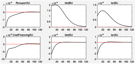
Figure 2. Responses of financial intermediates to confidence shock.
banking sector and shadow banking sector, respectively. Therefore, different forms of behavioral logic were observed in the economy. This study focused on the effect of confidence shocks, which greatly influence financial intermediaries. We found that:
1) Confidence is essential to economic development because it can affect the overall economy, thereby enabling the economy to grow greatly in terms of aspects such as output, consumption, and investment.
2) In the presence of a shadow banking system, increased confidence exerts a great effect on shadow banks and the sector supported by them. This effect increases overall economic volatility, leaving the economy somewhat vulnerable.
3) The shadow banking sector, driven by the confidence effect, squeezes the credit business of commercial banks. This substitution effect changes the overall economic structure.
These findings offer some profound policy implications and suggestions as well. When the market becomes optimistic, policymakers should pay more attention to the impact of shadow banking on the economy, since the expansion of debt is mostly contributed by this sector. Regulation of shadow banking should be strengthened. Also, the effect of confidence is crucial to the growth of shadow banking as well as the change in economic structure. This suggests that confidence effect should be considered in policy planning and the path of economic development. Multi-targeted monetary policy that takes confidence effect into consideration may be effective and efficient.
Although our model captures several features of shadow banking and reveals the substitution effect, regulation and multi-targeted monetary policy are not discussed in this paper. Therefore, a possible direction for future research is to add them into the analysis.
Conflicts of Interest
The authors declare no conflicts of interest regarding the publication of this paper.
Cite this paper
Cong, H. and Chen, Y. (2018) Effect of Confidence Shock on an Economy with a Shadow Banking System: Analysis Based on Dynamic Stochastic General Equilibrium Model. Theoretical Economics Letters, 8, 3285-3300. https://doi.org/10.4236/tel.2018.815203
References
- 1. Pozsar, Z. (2008) The Rise and Fall of the Shadow Banking System. Regional Financial Review, 44, 1-13.
- 2. Adrian, T. and Shin, H.S. (2009) The Shadow Banking System: Implications for Financial Regulation. Staff Report, Federal Reserve Bank of New York, No. 382. https://doi.org/10.2139/ssrn.1441324
- 3. FSB (2013) Global Shadow Banking Monitoring Report 2013. http://www.fsb.org/wp-content/uploads/r_131114.pdf
- 4. FSB (2011) Shadow Banking: Scoping the Issues. http://www.fsb.org/wp-content/uploads/r_110412a.pdf
- 5. Pozsar, Z., Adrian, T., Ashcraft, A.B. and Boesky, H. (2010) Shadow Banking. Staff Report, Federal Reserve Bank of New York No. 458.
- 6. Adrian, T. and Ashcraft, A.B. (2012) Shadow Banking: A Review of the Literature. Staff Report, Federal Reserve Bank of New York, No. 580.
- 7. Bernanke, B.S., Gertler, M. and Gilchrist, S. (1999) The Financial Accelerator in a Quantitative Business Cycle Framework. Handbook of Macroeconomics, 1, 1341-1393. https://doi.org/10.1016/S1574-0048(99)10034-X
- 8. Christiano, L., Motto, R. and Rostagno, M. (2010) Financial Factors in Economic Fluctuations. Working Paper Series, European Central Bank, No. 1192. https://www.ecb.europa.eu/pub/pdf/scpwps/ecbwp1192.pdf?d5356f67e3559baae7b37a12d911262b
- 9. Smets, F. and Wouters, R. (2002) An Estimated Stochastic Dynamic General Equilibrium Model of the Euro Area: International Seminar on Macroeconomics. Europ. Central Bank.
- 10. Verona, F., Martins, M.M.F. and Drumond, I. (2013) (Un)anticipated Monetary Policy in a DSGE Model with a Shadow Banking System (Bank of Finland Research Discussion Paper 4/2013).
- 11. Diamond, D.W. and Dybvig, P.H. (1983) Bank Runs, Deposit Insurance, and Liquidity. Journal of Political Economy, 91, 401-419. https://doi.org/10.1086/261155
- 12. Gorton, G., Metrick, A., Shleifer, A. and Tarullo, D.K. (2010) Regulating the Shadow Banking System [with Comments and Discussion]. Brookings Papers on Economic Activity, Brookings Institution Press, Washington DC, 261-312. https://doi.org/10.1353/eca.2010.0016
- 13. Ferrante, F. (2018) A Model of Endogenous Loan Quality and the Collapse of the Shadow Banking System. American Economic Journal: Macroeconomics, 10, 152-201. https://doi.org/10.1257/mac.20160118
- 14. Christiano, L.J., Eichenbaum, M. and Evans, C. L. (2005) Nominal Rigidities and the Dynamic Effects of a Shock to Monetary Policy. Journal of Political Economy, 113, 1-45. https://doi.org/10.1086/426038
- 15. Calvo, G.A. (1983) Staggered Prices in a Utility-Maximizing Framework. Journal of monetary Economics, 12, 383-398. https://doi.org/10.1016/0304-3932(83)90060-0
- 16. Erceg, C.J., Henderson, D.W. and Levin, A.T. (2000) Optimal Monetary Policy with Staggered Wage and Price Contracts. Journal of monetary Economics, 46, 281-313. https://doi.org/10.1016/S0304-3932(00)00028-3
- 17. Levin, A.T., Onatski, A., Williams, J.C. and Williams, N. (2005) Monetary Policy under Uncertainty in Micro-Founded Macroeconometric Models. NBER Macroeconomics Annual, 20, 229-287. https://doi.org/10.1086/ma.20.3585423
- 18. Chen, L., Lesmond, D.A. and Wei, J. (2007) Corporate Yield Spreads and Bond Liquidity. The Journal of Finance, 62, 119-149. https://doi.org/10.1111/j.1540-6261.2007.01203.x