Theoretical Economics Letters
Vol.07 No.04(2017), Article ID:76136,13 pages
10.4236/tel.2017.74049
Optimal (Under-)Pricing and Allocation of Publicly Provided Goods
David Scrogin
University of Central Florida, Orlando, FL, USA

Copyright © 2017 by author and Scientific Research Publishing Inc.
This work is licensed under the Creative Commons Attribution International License (CC BY 4.0).
http://creativecommons.org/licenses/by/4.0/


Received: February 25, 2017; Accepted: May 12, 2017; Published: May 15, 2017
ABSTRACT
This paper exploits the links between a private value distribution’s hazard rate, mean residual value, and eta functions in order to characterize posted- price rules for a public agency to allocate scarce units of an indivisible good under the utilitarian distributional objective of maximizing expected consu- mer surplus. Sufficient conditions on the monotonic and non-monotonic classes of the functions are established that identify either market assignment at the clearing price or lottery assignment with partial or complete under- pricing as the optimal allocation mechanism. The results are summarized across a wide range of parametric value distributions, and selected non-mono- tonic cases are evaluated numerically to determine the relative scarcity or abundance of the good necessary for market or non-market assignment to dominate.
Keywords:
Expected Consumer Surplus, Non-Market Mechanism, Lottery, Hazard Rate, Mean Residual Value

1. Introduction
Public agencies are commonly commissioned with allocating scarce units of indivisible goods and services over large numbers of individuals or households. Examples include assigning seats in schools, parcels of land and housing, access to medical services, immigration visas, and recreational privileges on publicly managed commons. An accompanying dilemma that agencies confront entails implementing an allocation mechanism to determine who will be awarded a unit and who will not. While expected revenues are maximized from allocating units by price or willingness to pay alone, agency objectives, laws and legislative mandates, or majority public preferences may lead agencies to deviate from competitive market assignment by under-pricing and allocating the units through a non- market mechanism, such as a lottery, queue or reservation system, or a merit or need-based assignment rule.
Several studies have investigated non-market allocation mechanisms in isolation and relative to market assignment or employed mechanism design to characterize optimal rules for allocating indivisible goods and services. In early work, [1] considered distributional and political economic aspects of rationing by queue, and [2] formalized a pseudo-market mechanism―the waiting-line auction―to characterize queuing behavior and equilibrium arrival times. [3] compared auctions, lotteries, and queues under deterministic demand and identified conditions for non-market assignment rules to be majority preferred. And [4] and [5] compared the expected efficiency of lotteries and queues under stochastic demand, whereby individual private valuations are drawn independently from a common distribution, and both concluded lotteries are superior if the good is relatively scarce and individual private values and time costs are sufficiently homogenous or negatively correlated.
In the mechanism design literature, [6] considered the case of two individuals with independent private valuations competing for a single unit of a good and demonstrated that expected net efficiency is maximized by random assignment if individuals incur sufficient signaling costs and the hazard rate of the distribution of individual private valuations is increasing. [7] also found random assignment to be optimal given an arbitrary number of ex ante identical individuals and a value distribution with an increasing hazard rate, whereas market assignment is optimal if sufficient screening costs are incurred by the agency and the hazard rate is decreasing. And [8] investigated the allocation problem when individual signaling costs are socially wasteful and the agency seeks to maximize expected social surplus. Consistent with [6] and [7] , lottery assignment is shown to be optimal under certain conditions on individual types and the value distribution’s hazard rate.
While the settings and approaches for investigating the market versus non- market assignment problem vary across the literature, the shape of the value distribution’s hazard rate function (monotonic or non-monotonic) has consistently proven informative and critical to the conclusions. The tradition continues in this paper, where the links are exploited between the hazard rate function and its close counterparts―the mean residual life (or value) function and [9] ’s eta function―in order to address the agency’s mechanism choice problem under the distributional objective of maximizing aggregate expected consumer surplus (ECS)1. From a symmetric independent private values framework it is shown that the optimal mechanism can be determined directly from the mean residual value function or indirectly from the hazard rate and eta functions, and sufficient conditions on each are established for market assignment or random (lottery) assignment with partial or complete under-pricing to be optimal2. The analysis extends results from [10] ’s study of the effects of price controls on consumer surplus in competitive markets and demonstrates that maximizing ECS may be consistent with the agency achieving alternative objectives in allocating units of indivisible goods and services, such as maximizing revenues, net efficiency, or distributional equity. The results are summarized across a wide range of parametric distributions, and selected non-monotonic cases are evaluated numerically to determine the relative scarcity or abundance of the good necessary for market or non-market assignment to dominate.
2. ECS Maximizing Allocation Rules
2.1. The Setting and Allocation Problem
An agency holds Q* units of an indivisible good to be distributed over N > Q* individuals, where N is assumed large and Q* may be small or large relative to N. Each individual possesses unit demand and a private valuation v for the good that is independently drawn from the interval [0, ∞) according to the distribution function F(v) with density . Q*, N, and F(v) are assumed commonly known, and each individual also knows his/her valuation but not the valuation of any other individual. Individual expected demand is then represented by the survival function F+(v) = 1 − F(v). That is, F+(v) is the probability an individual’s valuation is at least v or the probability the individual would be willing to purchase a unit if the price were v. Aggregate expected demand is NF+(v), and the expected market clearing price v* satisfies NF+(v) = Q*.
The agency’s objective in allocating Q* is to maximize aggregate expected consumer surplus by posting a uniform price p Î [0, v*] and randomly assigning units if excess demand exists. Individual i’s expected probability of acquiring a unit conditional upon a valuation vi Î [p, ∞) is and i’s expected consumer surplus is written:
(1)
Aggregate expected consumer surplus the agency seeks to maximize is obtained by multiply (1) by expected demand, and the pricing problem is written:
(2)
Given the value distribution and clearing price, the solution to (2) may be described by one of three mechanisms for allocating Q*. These will be referred to as market assignment at the clearing price p = v*, pure lottery assignment at price p = 0, and hybrid lottery assignment at a price p Î (0, v*).
To proceed, note the term in brackets in (1) and (2) is the individual expected consumer surplus if a unit could be purchased outright for p. That is, it is the difference between a price p and the individual mean private valuation conditional upon it being at least as large as p. The expression is the value distribution equivalent of a lifetime distribution’s mean residual life function, defined . For a lifetime random variable X, MRL(t) is the expected remaining life of the respective entity (e.g., a machine or individual) conditional upon its ‘surviving’ to time t. MRL(t) is a close counterpart of the hazard rate function and [9] ’s eta function , and all are long-standing workhorses in the reliability engineering and stochastic ageing literature (see e.g., [11] and [12] ). Denoting the value distribution’s mean residual value function by MRL(v) and its hazard rate and eta functions by HR(v) and ƞ(v), ECS(p) in (2) is then the product of Q* and MRL(v) evaluated at price p = v for v Î [0, v*]. That is, ECS(p) = Q*MRL(p).
The relationship between ECS(p) and MRL(v) is appealing for characterizing the solution to (2) because the shape of ECS(p) (monotonic or non-monotonic) is the same as that of MRL(v) for vÎ [0, v*] and because the shape of MRL(v) is implied directly by HR(v) and indirectly by ƞ(v) as shown by [9] [13] and [14] 3. Evaluation of HR(v) or ƞ(v) may then be sufficient for determining the optimal allocation mechanism. The results are formalized for monotonic and non-mo- notonic classes of MRL(v), HR(v), and ƞ(v) in the remainder of this section and selected cases are evaluated numerically in Section 3.
2.2. Results
In order to distinguish the monotonic and non-monotonic classes of MRL(v) from one another, let IMRL (DMRL) denote MRL(v) that is monotonic increasing (decreasing). That is, MRL(v) is IMRL (DMRL) if MRL'(v) > 0 (<0) for v Î [0, ∞). For the non-monotonic classes, let DIMRL (IDMRL) denote the case in which MRL(v) initially decreases (increases) to a minimum (maximum) at v1 Î (0, ∞) and then increases (decreases). That is, MRL(v) is DIMRL (IDMRL) if MRL(v1) = 0, MRL'(v) < 0 (MRL'(v) > 0) for v < v1, and MRL'(v) > 0 (MRL'(v) < 0) for v > v1. Further, as MRL'(v) = HR(v)MRL(v) − 1, it follows that at MRL(v)’s interior minimum or maximum, MRL(v1) = 1/HR(v1). The monotonic and non- monotonic classes of HR(v) and ƞ(v) will be similarly referenced below (e.g., IHR and DIHR).
Given ECS(p) = Q*MRL(p) if p = v, it is clear that ECS(p) is maximized by market (pure lottery) assignment of Q* if MRL(v) is IMRL (DMRL). If instead MRL(v) is non-monotonic, then ECS(p) may or may not be monotonic for p Î [0, v*) and information on the relative scarcity or abundance of the good is needed to determine the optimal mechanism directly from MRL(v) or indirectly from HR(v) and ƞ(v). To link HR(v) and ECS(p) through MRL(v) the following sufficient conditions from [13] and [14] are used:4
i) If HR(v) is IHR (DHR), then MRL(v) is DMRL (IMRL).
ii) If HR(v) is IDHR and f(0)μ< 1 (f(0)μ ≥ 1), then MRL(v) is DIMRL (IMRL).
iii) If HR(v) is DIHR and f(0)μ> 1 (f(0)μ ≤ 1), then MRL(v) is IDMRL (DMRL).
Monotonicity of HR(v) therefore implies monotonicity of MRL(v), whereas non-monotonicity HR(v) may or may not imply non-monotonicity of MRL(v). For linking ƞ(v) and ECS(p) through HR(v), sufficient conditions from [9] are used. Defining ε and δ, respectively, as and , the conditions are:
i) If ƞ(v) is I (D), then HR(v) is IHR (DHR).
ii) If ƞ(v) is DI and ε = 0 or δ < 1 (ε = ∞ or δ > 1), then HR(v) is IHR (DIHR).
iii) If ƞ(v) is ID and ε = 0 or δ < 1 (ε = ∞ or δ > 1), then HR(v) is IDHR (DHR).
Monotonicity of ƞ(v) therefore implies monotonicity of HR(v) and of MRL(v) by transitivity, whereas if ƞ(v) is non-monotonic, then HR(v) and MRL(v) may or may not be non-monotonic. While the above conditions are used here for characterizing optimal allocation rules, they have proven invaluable for determining the shape of MRL(t) in reliability engineering and stochastic ageing studies because MRL(t) typically does not appear in closed form (see e.g., [11] ).
The solution to (2) is given first in Proposition 1 and Corollary 1 for cases of HR(v) and ƞ(v) that imply MRL(v) that is monotonic, followed by the cases of non-monotonic MRL(v) in Propositions 2 and 3.
Proposition 1: Given Q*, N, and F(v):
i) If HR(v) is DHR (IHR), then ECS(p) is maximized by market (pure lottery) assignment of Q*.
ii) If HR(v) is IDHR and μf(0) ≥ 1 (DIHR and μf(0) ≤ 1), then ECS(p) is maximized by market (pure lottery) assignment of Q*.
Proof: i) If HR(v) is DHR (IHR), then MRL(v) is IMRL (DMRL). Therefore, ECS(v*) > ECS(p) for p Î [0, v*) (ECS(0) > ECS(p) for p Î (0, v*]) and ECS(p) is maximized by market (pure lottery) assignment of Q*.
ii) If HR(v) is IDHR and μf(0) ≥ 1 (DIHR and μf(0) ≤ 1), then MRL(v) is IMRL (DMRL). Therefore, ECS(v*) >ECS(p) for pÎ [0, v*) (ECS(0) >ECS(p) for p Î (0, v*]) and ECS(p) is maximized by market (pure lottery) assignment of Q*.
Distributions for which Proposition 1 applies (and Propositions 2 and 3 below) are reported in Table 1. If private values are Pareto distributed (see [10] for a detailed example) or exponential-geometric distributed, then MRL(v) is IMRL and ECS(p) is maximized by market assignment of Q*, and if private values are uniform, truncated normal, or Gompertz-Makeham distributed, then MRL(v) is DMRL and ECS(p) is maximized by allocating Q* by pure lottery. If instead values are Weibull or gamma distributed, then market or pure lottery assignment could be optimal as MRL(v) is either IMRL or DMRL.
Corollary 1 follows immediately from Proposition 1 and [9] ’s sufficient condi-

Table 1. Allocation Mechanisms that Maximize ECS(p) for Parameteric Value Distributionsa.
aThe distributions and their properties are discussed in [11] [12] or [17] .
tions on ƞ(v) discussed above.
Corollary 1: Given Q*, N, and F(v):
i) If ƞ(v) is D(I), then ECS(p) is maximized by market (pure lottery) assignment of Q*.
ii) If η(v) is DI (ID) and ε = 0 or δ < 1 (ε = ∞ or δ > 1), then ECS(p) is maximized by pure lottery (market) assignment of Q*.
Proof: The results follow by transitivity from Proposition 1 and [9] ’s sufficient conditions on η(v) for HR(v) to be DHR or IHR, implying MRL(v) is IMRL or DMRL, respectively.
In the remaining cases, HR(v) implies MRL(v) is non-monotonic. A graphical depiction of HR(v) and MRL(v) that are i)IDHR and DIMRL and ii)DIHR and IDMRL appear in Figure 1 and Figure 2, respectively. Included are MRL(v) and 1/HR(v). From Figure 1, if the clearing rate v* is such that MRL(v*) > MRL(vμ) = μ, then F+(v*) < F+(vμ) and ECS(p) is maximized by market assignment, and if MRL(v*) < MRL(vμ)= μ, then F+(v*) >F+(vμ) and ECS(p) is maximized by pure lottery assignment. From Figure 2, if v* > v1 then MRL(v*) < MRL(v1), F+(v*) < F+(v1), and ECS(p) is maximized by allocating Q* by hybrid lottery at price p = v1; otherwise, market assignment of Q* is optimal.
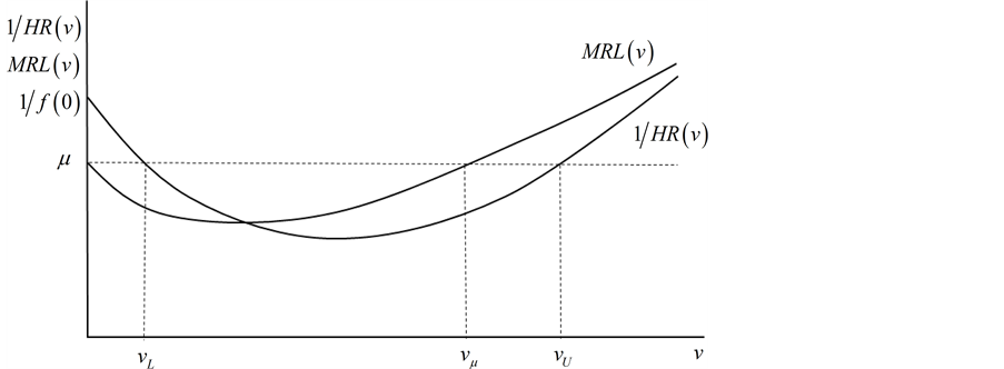
Figure 1. Example of Non-monotonic HR(v) and MRL(v) for Proposition 2.
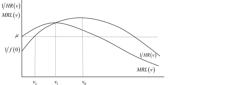
Figure 2. Example of Non-monotonic HR(v) and MRL(v) for Proposition 3.
Figure 1 and Figure 2 also indicate that the optimal mechanism can be determined from evaluation of HR(v) and μ if v* is sufficiently scarce or abundant. The results are formalized in Proposition 2 for HR(v) implying DIMRL and in Proposition 3 for HR(v) implying DIMRL.
Proposition 2: Given HR(v) that is IDHR and μf(0) < 1:
i) If HR'(v*) > 0 and 1/HR(v*) ≥ μ, then ECS(p) is maximized by pure lottery assignment of Q*.
ii) If HR'(v*) < 0 and 1/HR(v*) ≥ μ, then ECS(p) is maximized by market assignment of Q*.
iii) If , then ECS(p) is maximized by pure lottery assignment of Q*.
Proof: In all cases, if HR(v) is IDHR and μf(0) < 1, the MRL(v) is DIMRL.
i) As MRL'(v) < 0 if HR'(v) > 0 and 1/HR(v) ≥ μ, it follows that if HR'(v*) > 0 and 1/HR(v*) ≥ μ, then μ > MRL(v*). Therefore, ECS(0) > ECS(p) for p Î (0, v*] and ECS(p) is maximized by pure lottery assignment of Q*.
ii) If HR'(v*) < 0 and 1/HR(v*) ≥ μ, then MRL(v*) > μ. It follows that ECS(v*) > ECS(p) for p Î [0, v*) and ECS(p) is maximized by market assignment of Q*.
iii) From [16] , if the latter limit is finite. Therefore,
if . It follows that ECS(0) > ECS(p) for p Î (0, v*] and ECS(p) is maximized by pure lottery assignment of Q*.
Figure 1 depicts cases i and ii of Proposition 2.5 Case i applies to the lower interval v Î [0, vL]. As HR'(v) > 0 and 1/HR(v) ≥ μ, it follows that μ > MRL(v). Therefore, if Q* is sufficiently abundant such that v* ≤ vL, then ECS(0) > ECS(v*), and ECS(p) is maximized by allocating Q* by pure lottery. For case ii, as HR'(v) < 0 and 1/HR(v) ≥ μ in the upper interval v Î [vU, ∞), it follows that MRL(v) > μ. Therefore, if Q* is sufficiently scarce such that v* ≥ vU, then ECS(v*) > ECS(0) and market assignment is optimal. Similar to Proposition 1, examples of distributions for which Proposition 2 applies are reported in Table 1. Included are the lognormal, inverse Gaussian, log-logistic, and Burr XII distributions and variants of the Weibull distribution.
Lastly, the case in which HR(v) implies MRL(v) that is IDMRL is covered in Proposition 3.
Proposition 3: Given HR(v) that is DIHR and μf(0) > 1:
i) If HR'(v*) < 0 and 1/HR(v*) ≤ μ, then ECS(p) is maximized by market assignment of Q*.
ii) If HR'(v*) ≥ 0, then ECS(p) is maximized by hybrid lottery assignment of Q*.
Proof: In both cases, if HR(v) is DIHR and μf(0) > 1, then MRL(v) is IDMRL.
i) If HR'(v*)< 0 and 1/HR(v*) ≤ μ, then v* < v1. As Q* > NF+(v) for v>v* and MRL'(v) > 0 for v < v1, it follows that ECS(v*) > ECS(p) for p Î [0, v*) and ECS(p) is maximized by market assignment of Q*.
ii) If HR'(v*) ≥ 0, then v* > v1 and MRL(v) > MRL(v*) for v Î [v1, v*). Therefore, ECS(p) > ECS(v*) for p Î [v1, v*) and ECS(p) is maximized by hybrid lottery assignment of Q*.
Results from Proposition 3 are depicted in Figure 2. Case i applies to the interval v Î [0, vL]. As HR'(v) < 0 and 1/HR(v) ≤ μ it follows that MRL(v) > μ and MRL'(v) > 0. Therefore, if the scarcity of Q* is such that v* ≤ vL, then ECS(0) < ECS(v*), and ECS(p) is maximized by selling Q* outright. For case ii, as MRL'(v) < 0 for v Î (v1, ∞), if HR'(v*) ≥ 0 (or v* ≥ v0) then MRL(v0) ≥ MRL(v*). It follows that MRL(v) > MRL(v*) for some values in the interval (0, v*). Therefore, if Q* is sufficiently abundant such that v* ≥ v0, then ECS(p) attainable from allocating Q* by hybrid lottery exceeds that from market assignment. Table 1 report several distributions for which Proposition 3 applies. Included are the beta and exponential power distributions and variants of the Weibull distribution.
3. Numerical Examples
As shown above, while the allocation mechanism that maximizes ECS(p) is independent of Q* if MRL(v) is monotonic (Proposition 1), information on the relative scarcity or abundance of the good is needed to determine the optimal mechanism if MRL(v) is non-monotonic (Propositions 2 and 3). To demonstrate, two of the distributions reported in Table 1 are evaluated numerically. In the first, private values are assumed log-logistic distributed. MRL(v) is DIMRL for certain parameter values and ECS(p) is maximized either by market or pure lottery assignment (see Proposition 2 and Figure 1). In the second, private values are assumed beta distributed. MRL(v) is IDMRL for certain parameter values and ECS(p) is maximized either by market or hybrid lottery assignment (see Proposition 3 and Figure 2).
3.1. Log-Logistic Distribution
The survival and hazard rate functions of the log-logistic distribution are given by:
(3)
where α > 0 and β > 0. Derivation of MRL(v) yields:
(4)
where F(v) = 1 − F+(v), B(1/β, 1 − 1/β) is the beta function, BF(v)(1/β, 1 − 1/β) is the incomplete beta function, and (see [11] ). Despite the complexity of MRL(v), if β > 1, then HR(v) is IDHR and μf(0) − 1 < 0 and therefore MRL(v) is DIMRL.
To determine the optimal mechanism directly from MRL(v) or indirectly from HR(v) and μ (Proposition 2), and referencing Figure 1, if MRL(v*) > MRL(vμ) = μ, then F+(v*) < F+(vμ) and ECS(p) is maximized by selling Q* outright. If instead MRL(v*) < MRL(vμ) = μ, then F+(v*) > F+(vμ) and ECS(p) is maximized by pure lottery. F+(vμ) is calculated from (3) and (4) across a range of parameter values and compared against F+(v*) = Q*/N (or NF+(v*) = Q*) to determine from MRL(v) whether market or pure lottery assignment is dominant.
For evaluation of Proposition 2, if 1/HR(v*) > 1/HR(vL) = μ and HR'(v*) > 0, then F+(v*) > F+(vL) and MRL(v*) < MRL(v) for v Î [0, v*). It follows that ECS(p) is maximized by allocating Q* by pure lottery. If instead 1/HR(v*) > 1/HR(vU) = μ and HR'(v*) < 0, then F+(vU) > F+(v*) and MRL(v*) > MRL(v) for v Î [0, v*). Therefore, ECS(p) is maximized by selling Q* outright. F+(vL) and F+(vU) are calculated and compared against F+(v*) = Q*/N to determine the relative scarcity or abundance of the good for the mechanism to be identified from HR(v) and μ.
The first half of Table 2 reports F+(vμ), F+(vL), F+(vU), and the Gini coefficient for the log-logistic distribution across a range of (α, β) values. The Gini coefficient indicates that individual private values become increasingly homogenous as β increases from 1. Considering F+(vμ), the results indicate and . It follows that given the relative scarcity of the good, market (pure lottery) assignment will tend to dominate as β → 1 (β → ∞). For example, if β ≤ 2 then F+(vμ) ≥ 0.50. Therefore, MRL(v*) > μ and ECS(v*) > ECS(0) if F+(v*) < 0.50. It follows that market assignment dominates pure lottery assignment if Q* is less than half of N. In contrast, if β ≥ 3 then F+(vμ) < 0.10, so pure lottery assignment will dominate if N is less than ten times greater than Q*.
Table 2. Ranges of the Log-logistic and Beta Distributions for Maximizing ECS(p) by Market, Pure Lottery, or Hybrid Lottery Assignmenta.
aFrom F+(v) = 1 − F(v), where F(v) is the cumulative distribution function, F+(vμ) references MRL(vμ) = μ; F+(vL) references 1/HR(vL) = μ; similarly, F+(vU) references 1/HR(vU) = μ; F+(v0) references HRʹ(v0) = 0; and F+(v1) references MRLʹ(v1) = 0. The values and equalities also appear in Figure 1 and Figure 2.
3.2. Beta Distribution
In contrast to the log-logistic distribution, the upper bound of the beta distribution is finite and the survival and hazard rate functions do not appear in closed form. The functions may be written:
(5)
where α > 0 and β > 0, and B(α, β) and Bv(α, β) are the beta function and incomplete beta function, respectively. Derivation of MRL(v) yields:
(6)
where . [15] showed that HR(v) is DIHR and MRL(v) is IDMRL for α < 1.
To determine the mechanism that maximizes ECS(p) directly from MRL(v), and referencing Figure 2, note that MRL(v) attains an interior maximum atv1, so if v1 ≥ v* then F+(v*) ≥ F+(v1) and ECS(p) is maximized by market assignment of Q*. If insteadv1 < v* then F+(v*)
For evaluating Proposition 3, if 1/HR(v*) < 1/HR(vL) = μ and HR'(v*) < 0, then F+(v*) > F+(vL) and MRL(v*) > MRL(v) for v Î [0, v*). It follows that ECS(p) is maximized by selling Q* outright. If instead 1/HR(v*) < 1/HR(v0) and HR'(v) > 0, then F+(v*)
6The Gini coefficient of the beta distribution is given by (α/2)B(α + β, α + β)/(B(α, α)B(β, β)).
The second half of Table 2 reports F+(v1), F+(vL), F+(v0), and the Gini coefficient across a range of (α, β) values6. In contrast to the log-logistic distribution, the homogeneity of individual private values is relatively constant across the cases considered as indicated by the Gini coefficients. Referencing F+(v1), the results indicate the interior maximum of MRL(v) is located well within the upper and lower bounds of the distribution, with F+(v1) ranging from 0.66 to about 0.40. As ECS(p) is maximized by hybrid lottery assignment at price p = v1 if F+(v1) > F+(v*) and by market assignment at p = v* if F+(v1) ≤ F+(v*), it follows that across the cases reported in Table 2 the hybrid lottery is optimal if Q* is less than fourth tenths of N and market assignment is optimal if Q* is at least two thirds as large as N.
The results in Table 2 also identify the relative scarcity or abundance of Q*needed for the optimal allocation mechanism to be determined from HR(v) and μ, as formalized in Proposition 3. As F+(vL) ranges from 0.73 to 0.63 and F+(v0) ranges from about 0.40 to 0.22, it follows that allocation of Q* by hybrid lottery is optimal over all cases in Table 2 if F+(v*) < 0.22, or N is at least five times greater than Q*, whereas market assignment is optimal if F+(v*)> 0.73, or Q* is at least three-fourths as large as N. Overall, in settings in which the agency has a limited number of units to be allocated over a large population of individuals, if private values are beta distributed with α < 1, then the expected consumer surplus from screening low-valued individuals by posting a non-zero price and assigning units by lottery will exceed that resulting from selling the units outright.
4. Conclusions
This paper contributes to the growing body of literature investigating the performance, merits, and shortcomings of non-market allocating mechanisms against market-based benchmarks. A framework was developed for characterizing optimal posted-price mechanisms for a public agency confronted with the problem of allocating units of an indivisible good or service under the utilitarian distributional objective of maximizing aggregate expected consumer surplus. From a setting of symmetric independent individual private valuations and survival function representations of individual and aggregate demand, the optimal allocation mechanism could be determined from direct evaluation of the value distribution’s mean residual value function or indirectly from the hazard rate and [9] ’s eta function.
Monotonicity of any of the three functions was shown to be sufficient to identify either market assignment or pure lottery assignment as being optimal, whereas information on the relative scarcity or abundance of the good may or may not be necessary to determine the optimal mechanism and degree of under- pricing for the non-monotonic classes of the functions. The results also provide a simple means by which to determine the optimal mechanism given distributional assumptions regarding individual private valuations and allow for direct comparison to outcomes in the design literature established in terms of the hazard rate function. The current work can be extended in several dimensions, two of which include the introduction of a revenue target for the agency and the characterization of the optimal mechanism when units of the good can be partitioned and allocated through a mixture of market and non-market mechanisms.
Acknowledgements
I am grateful for the helpful comments on an earlier version of the work by seminar participants at the University of Central Florida and by an anonymous reviewer. Any errors are my own.
Cite this paper
Scrogin, D. (2017) Optimal (Under-)Pricing and Allocation of Publicly Provided Goods. Theoretical Economics Letters, 7, 683-695. https://doi.org/10.4236/tel.2017.74049
References
- 1. Barzel, Y. (1974) A Theory of Rationing by Waiting. The Journal of Law and Economics, 17, 73-95. http://www.jstor.org/stable/724744
- 2. Holt, C.A. and Sherman, R. (1982) Waiting-Line Auctions. Journal of Political Economy, 90, 280-294. http://www.jstor.org/stable/1830293
- 3. Boyce, J.R. (1994) Allocation of Goods by Lottery. Economic Inquiry, 32, 457-476. https://doi.org/10.111/j.1465-7295.1994.tb01343.x
- 4. Taylor, G.A., Tsui, K.K. and Zhu, L. (2003) Lottery or Waiting-line Auction? Journal of Public Economics, 87, 1313-1334. https://dx.doi.org/10.1016/S0047-2727(01)00196-7
- 5. Koh, W.T.H., Yang, Z. and Zhu, L. (2006) Lottery Rather than Waiting-Line Auction. Social Choice and Welfare, 27, 289-310. https://doi.org/10.1007/s00355-006-0134-y
- 6. Yoon, K. (2011) Optimal Mechanism Design When Both Allocative Inefficiency and Expenditure Inefficiency Matter. Journal of Mathematical Economics, 47, 670-676. https://dx.doi.org/10.1016/j.jmateco.2011.09.002
- 7. Condorelli, D. (2013) Market and Non-Market Mechanisms for the Optimal Allocation of Scarce Resources. Games and Economic Behavior, 82, 582-591. https://dx.doi.org/10.1016/j.geb.2013.08.008
- 8. Chakravarty, S. and Kaplan, T.R. (2013) Optimal Allocation without Transfer Payments. Games and Economic Behavior, 77, 1-20. https://dx.doi.org/10.1016/j.geb.2012.08.006
- 9. Glaser, R.E. (1980) Bathtub and Related Failure Rate Characterizations. Journal of the American Statistical Association, 75, 667-672.
- 10. Bulow, J. and Klemperer P. (2012) Regulated Prices, Rent Seeking, and Consumer Surplus. Journal of Political Economy, 120, 160-186.
- 11. Lai, C.D. and Xie, M. (2006) Stochastic Ageing and Dependence for Reliability. Springer Science+ Business Media, Inc., New York.
- 12. Marshall, A.W. and Olkin, I. (2007) Life Distributions: Structure of Nonparametric, Semiparametric and Parametric Families. Springer Science + Business Media, LLC, New York.
- 13. Bryson, M.C. and Siddiqui, M.M. (1969) Some Criteria for Aging. Journal of the American Statistical Association, 64, 1472-1483.
- 14. Gupta, R.C. and Akman, H.O. (1995) Mean Residual Life Functions for Certain Types of Non-monotonic Ageing. Communications in Statistics-Stochastic Models, 11, 219-225. https://dx.doi.org/10.1080/15326349508807340
- 15. Ghitany, M.E. (2004) The Monotonicity of the Reliability Measures of the Beta Distribution. Applied Mathematics Letters, 17, 1277-1283.https://dx.doi.org/10.1016/j.aml.2003.12.007
- 16. Bradley, D.M. and Gupta, R.C. (2003) Limiting Behavior of the Mean Residual Life Function. Annals of the Institute of Statistical Mathematics, 55, 217-226.
- 17. Bagnoli, M. and Bergstrom T. (2005) Log-Concave Probability and Its Applications. Economic Theory, 26,445-469. https://doi.org/10.1007/s00199-004-514-4
NOTES
1For a given assignment of the good, consumer surplus is the difference between the sum of the private valuations of the recipients and the price each incurs for a unit of the good. Consumer surplus then appears in expectation because the agency is assumed to know the distribution of individual private valuations but not the valuation of any particular individual and because units of the good are allocated by lottery if price is set below the clearing rate. Further, as the price is posted by the agency prior to assigning the units, the randomness of consumer surplus over the set of possible assignments is not due to price uncertainty.
2The hazard rate and eta function characterizations of the solution to the mechanism choice problem are appealing for evaluating particular value distributions (e.g., uniform, Pareto, Weibull, etc.) because unlike the mean residual value function, the hazard rate and eta functions commonly appear in closed form.
3Relations between MRL(v), HR(v), and η(v) can be seen by noting that MRL'(v) = HR(v)MRL(v) − 1, MRL'(v) = HR'(v)MRL(v) + HR(v)MRL'(v), and HR'(v) >/=/< 0 if η(v) >/=/< 1/HR(v).
4 [15] showed that conditions i-iii also hold if the distribution has a finite upper bound.
5Case iii would appear in place of case ii in Figure 1 if .
6The Gini coefficient of the beta distribution is given by (α/2)B(α + β, α + β)/(B(α, α)B(β, β)).