Theoretical Economics Letters
Vol.4 No.2(2014), Article ID:43525,7 pages DOI:10.4236/tel.2014.42021
A Model of Room Rentals in a Seasonal Hotel Illustrating Monopolistic Competition
Gerald Aranoff
Ariel University Center of Samaria, Bnei Brak, Israel
Email: garanoff@netvision.net.il
Copyright © 2014 by author and Scientific Research Publishing Inc.
This work is licensed under the Creative Commons Attribution International License (CC BY).
http://creativecommons.org/licenses/by/4.0/


Received 24 December 2013; revised 24 January 2014; accepted 31 January 2014
ABSTRACT
We illustrate monopolistic competition with an original model of hotel rooms for daily rental that has peak and off-peak demand periods. There are two types of hotels, hotelK and hotelL, each having linear total costs with absolute capacity limits. HotelsK are static efficient since they operate with low MC. They are open year-around and always at full capacity. HotelsL are output flexible since they operate with low FC. They open only in the peak-demand periods. We show, under conditions of the model, that the added cost to supply irregular demand should be small because of hotelsL low FC. We show, under the conditions of the model, that the added gain in consumer surplus in increasing the irregularity should be large because consumers will be switching some consumption from off-peak to peak periods.
Keywords:Monopolist Competition; Demand Fluctuations; Marginal Cost Pricing; Consumer Surplus; Cost Curve

1. An Original Theoretical Model of Monopolist Competition
We illustrate monopolist competition with an original theoretical model of hotel rooms available for rent on a daily basis. The product is differentiated in that hotel rooms offered for daily rental differ in location, physical aspects and service. We assume fluctuating demand, with a peak season, for almost two months, and an off-peak season, for the balance of the year. We assume hotels set two prices, one for the peak season and one for the offpeak season. We assume no price collusion among hotels. We assume hotels know the consumer-demand schedules for their room rentals. We assume zero expected profits for all hotels in long-run equilibrium. Initially we assume SRMC pricing.
2. Room Rentals in a Seasonal Hotel: The Supply Side
We assume a single homogeneous product,  , hotel rooms rented at a daily rate. We assume ease of entry of new hotels. We assume two states of demand,
  and
and , off-peak and peak, each with a likelihood, where the likelihoods add to one. There are two types of hotels, hotelK and hotelL, each having linear total costs with absolute capacity limits. Hotels have durable and specific assets, and linear short-run total-cost curves with absolute capacity limits. Per-room per-day variable-operating cost
 , per-room per-day capacity costs
  (fixed costs per month divided by maximum rooms available rate per month) and capacity per hotel
  (maximum rooms available). We envision investors and managers walking into a hotel construction store that has two shelves: each with a model hotel
  that costs, say, $1,000,000 to build. On one shelf is a model of hotelK and on the other shelf is a model hotelL (see Figure 1). Investors or entrepreneurs can order any multiple or fraction of the model hotel. No economies of scale exist for hotels. Thus the long-run marginal cost (LRMC) and longrun average cost (LRAC) for hotels in the hotel construction store are horizontal.
2.1. Key Assumptions
The key assumptions of the model are:
A1: ,
,  , and
, and  as in Figure 2. The curves in Figure 2 must cross or else the lower one will dominate.
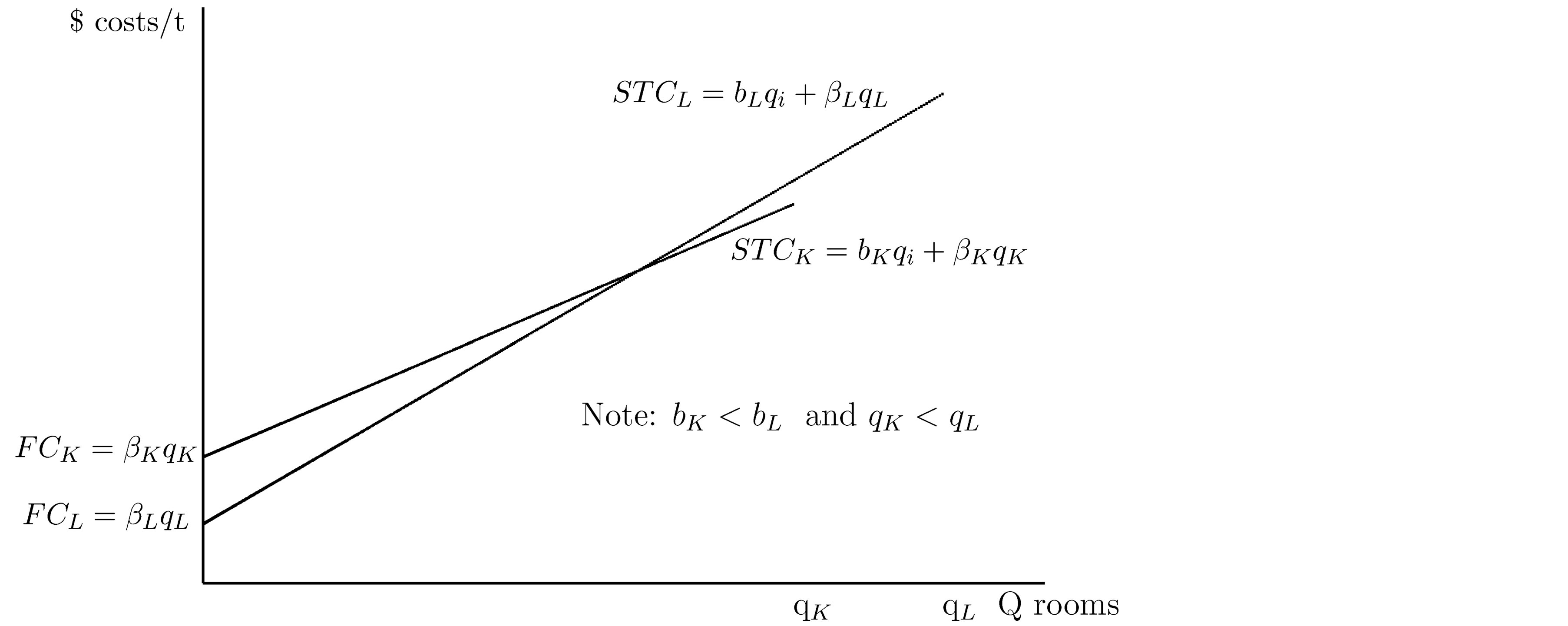
Figure 1. HotelK and HotelL SR total-cost curves.
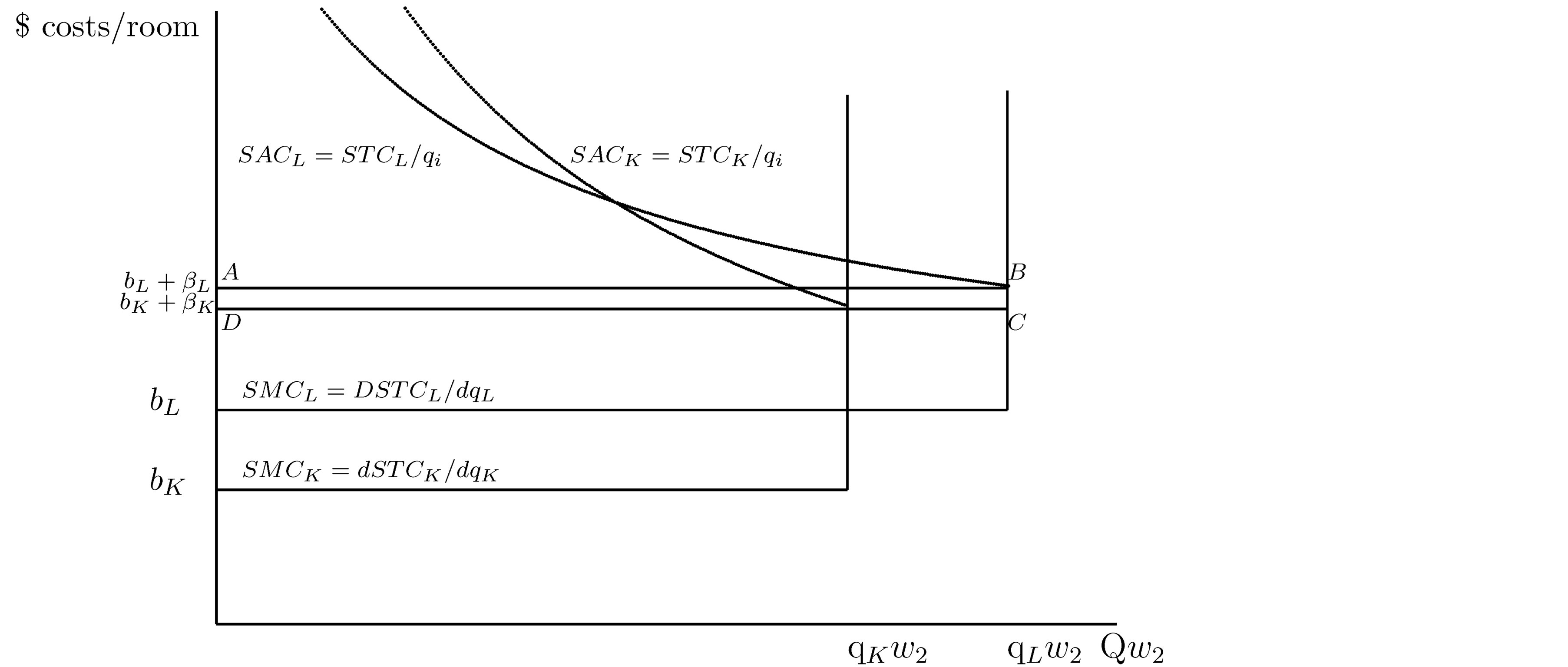
Figure 2. HotelL added cost of supplying irregular demand: ABCDw2.
A2: Demand fluctuates with frequencies,  in off-peak and
  in peak and
 .
.
A3: We assume SRMC (short-run marginal-cost) pricing behavior. With linear TC functions and SRMC pricing, hotels will operate at either 0% or 100%.
A4: We assume market prices in off-peak times :
:  and market prices in peak times
 :
: . Thus hotel
 operates at capacity at all times, while hotelL shuts down in
  and operates at capacity in
 . Total rooms rented in the industry in the off-peak period is
  where
where . Total rooms rented in the industry in the peak period is
  where
where .
.
A5: Long-run equilibrium requires zero expected profits for both hotels.
2.2. Objective of Proposition 1
We prove in the following proposition the conditions of indifference for investors to choose between hotelk and hotelL in LR equilibrium.
2.3. Proposition I
Proposition 1 Under assumptions A1 through A5 with both hotels used in long-run equilibrium, then it must be true:
 . (1)
. (1)
If  (that is, the left-side inequality is violated) then only hotel
 will be used. If
 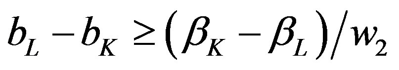 (that is, the right-side inequality is violated) then only hotelK will be used.
Proof: Applying the zero profit condition to hotelK:
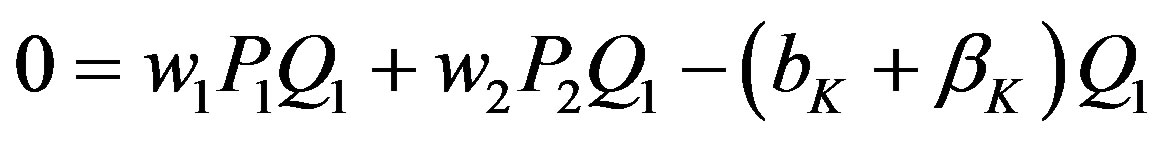 (2)
(2)
This gives us:
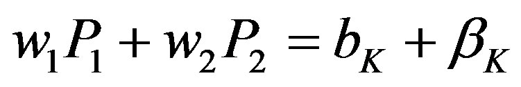 (3)
(3)
Applying the zero profit condition to hotelL:
 (4)
(4)
This gives us:
 (5)
(5)
Equations (3) and (5) can be combined:
 (6)
(6)
For hotelsL to shut-down in the off peak period requires , assumption A4. If
  then, strictly speaking, hotels
 are indifferent to operating and some may be operating. Using Equation (6), this requires:
 (7)
(7)
Since , We can write:
 (8)
(8)
which is the asserted left-side inequality condition:
 (9)
(9)
By assumption A4,  , hotelsK to earn a positive contribution margin or all hotels, even hotelsK, would choose to shut-down in
 . Further,
  because if
 , then positive expected profits to the owners of hotelsK would emerge. Thus
 (10)
(10)
yields the right-side inequality condition assertion.
2.4. Left-Side and Right-Side Inequality Conditions
The left-side condition in (1) is that . If one more room is needed in both peak and off-peak times, the total cost over the cycle of a 1 room capacity hotel over the cycle is
  since
since . A price of
  will exactly cover costs of one extra room operating in both periods. We suggest calling this condition that hotel
 be more static efficient, in the sense of Clark’s use of the term static in that there are no business cycles [1] [2] 1.
The right-side condition in (1) is that
 .
.
Assume we need one more room over the cycle only to meet peak demand. A price of  will exactly cover costs of one extra room over the cycle operating only in high-demand.
The right-hand condition is that where production is used only in high-demand times, hotelL is superior. The right-hand condition requires that SACL be flatter shaped than SACK. We define output flexibility as the relative flatness of the SAC curve. We suggest calling this condition that hotelL be more output-flexible efficient2.
2.5. HotelL Added Cost of Supplying Irregular Demand: ABCDw2
If demand for hotel rooms were static with no irregularities, then firms would choose only hotelK and 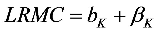 . Demand for hotel rooms is irregular in the model, fluctuating between
  and
and . The added cost of supplying irregular demand in the model is borne entirely by hotelL where
  .
.
Thus, a measure of added cost of supplying irregular demand in the model would be the expected rooms to meet peak demand × the difference in SRAC between the two hotels, or: . See Figure 2 which shows the added cost of supplying irregular demand for a single hotelL (rectangle ABCDw2).
Rectangle ABCDw2 shows, in the model of the paper, the added cost to have output-flexible hotelL, available only to provide for the excess peak over off-peak demand3.
3 Room Rentals in a Seasonal Hotel: The Demand Side
3.1. Definition of the Model and Its Terms and Assumptions
There are two groups in our hypothetical society: Suppliers (owners-managers of hotels) and consumers (households who rent hotel rooms). Consumers rent rooms in a free market on a daily basis from various hotels where each hotel posts its prices. Consumers pay the lowest price per-room per-day in the local market. The intersection of this price with the consumer demand schedules (off-peak and peak) determine the quantity of rooms the consumers order.
Consumers have a fixed budget for room rentals expenditures. They are price sensitive in renting rooms, in the sense that consumers will rent more rooms at a lower market price and less rooms at a higher market price. Consumers pay market price times quantities purchased,  (total revenue to suppliers equals market price times quantities).
The demand curve shows the maximum quantities consumers would be willing to purchase at various prices. The assumption is that the demand curve is downward sloping, meaning that consumers would be willing to rent more rooms daily if prices were lower, all else being the same. The area under the demand curve up to the point of quantities of market purchases shows the value to the consumer.
Figure 3 shows a geometric demonstration with varying pricing (alternative A) versus fixed pricing (alternative B) with fluctuating D functions, off-peak period and peak period each with its associated . Let D1 be consumer demand for rooms during off-peak periods, the great majority of the year, say 6/7th of the year.
Using hypothetical numbers to make the economic concepts clearer, point K could be that, at a market price of $36 per room per day consumers are willing to rent 35 rooms per day. Point H might be that at a market price
Figure 3.  pricing adds consumer surplus:
 .
.
of $33 per room per day consumers are willing to rent 37 rooms per day.
Let D2 be consumer demand for daily room rentals on the peak period. Using hypothetical numbers to illustrate, point D could be that, at a market price of $51.9 per room per day consumers are willing to rent 42 rooms per day. Point J could be that, at a market price of $36 per room per day consumers are willing to rent 54 rooms per day.
The demand curve , off-peak period demand, occurs with frequency,
  , 6/7. The demand curve
 . Peak period demand, occurs with frequency,
  , 1/7.
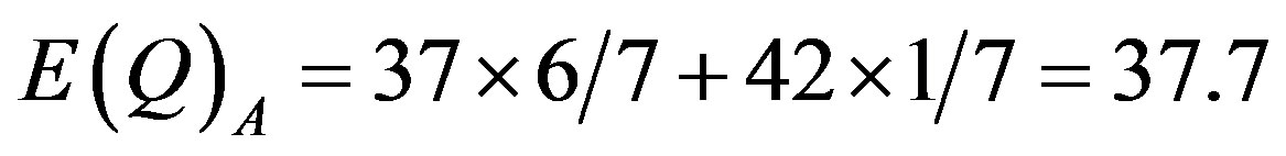
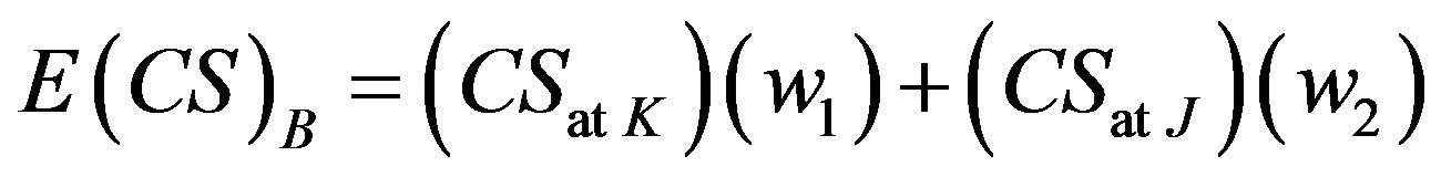
We define consumer surplus as the area under the demand curve and above the price line. We define expected values, E, as the sum of each outcome times its expected value. Using the illustrated numbers for points H and D, the market equilibrium points for pricing rule A, varying prices, we can calculate , expected total revenue, and
 , expected quantities, as follows:

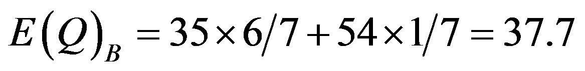
Using the illustrated numbers for points K and J, the market equilibrium points for pricing rule B, fixed prices, we can calculate , expected total revenue, and
 , expected quantities, as follows:

3.2. Objective of Proposition II
We prove in the following proposition that consumer surplus is necessarily larger in an arrangement where consumers get more rooms for the peak period at the cost of less rooms for the off-peak periods whereby consumers pay the same amount and rent the same number of rooms over the year. We show graphically this increase in consumer surplus. This becomes a maximum willingness for consumers to pay suppliers for that arrangement.
We assume that suppliers are willing to offer rooms daily according to two alternative pricing schemes: a fixed price,  , at all times, versus
  for off-peak periods and
  for the peak period. We have two basic assumptions in the model: according to both pricing schemes total payments over the week are the same and total food purchases are the same.
3.3. Proposition II
Proposition 2 A comparison of alternative pricing schemes, A: varying prices, versus B: fixed prices, under conditions of shifting downward-sloping demand curves shows  and rises as demand elasticity rises assuming
 (11)
(11)
and
 (12)
(12)

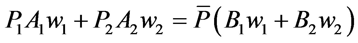
Proof: By definition of :
:
 (13)
(13)
and
 (14)
(14)
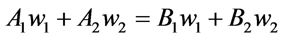
By definition of :
:
 (15)
(15)
and
 (16)
(16)
By definition of :
:
 (17)
(17)
and
 (18)
(18)
By assumption (11), we can state:
 (19)
(19)
By assumption (12), we can state:
 (20)
(20)
Combining assumptions (11) and (12):
 (21)
(21)
Rearranging:
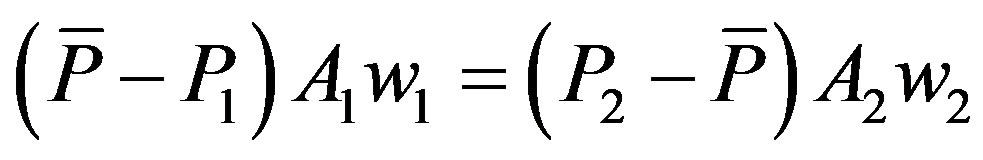 (22)
(22)
Using the letters of the Figure 3:
 (23)
(23)
We can state:
 (24)
(24)
Rearranging:
 (25)
(25)
We can state:
 (26)
(26)
Using the results of Equation (23), We can state:
 (27)
(27)
Thus,  must be greater than zero, providing that price elasticities of the demand curves are not zero. At zero price elasticity
  and
and  and therefore areas
  and
and  each equals zero.
  rises as price elasticity rises, since the areas of
  increase with more elastic demand curves.
3.4.  Pricing Adds Consumer Surplus:
 represents the gain in consumer surplus with fixed pricing over varying pricing that gives the same expected TR to suppliers and same expected Q to consumers. Theoretically
  is a maximum willingness to pay for an arrangement of an increase in irregularity. This is a beginning of constructing a demand schedule for irregularity. The increase in irregularity is going from
  to
to . We could test maximum willingness to pay to increase irregularity further or for a lesser degree of increase irregularity. We could explore the effects on consumer surplus with alternative pricing schemes that expected payments rise or expected Q falls.
4. Conclusions
We present here an original model of room rentals in a seasonal hotel as an example of monopolistic competition. Each hotel has differences of location, physical aspects and services offered. Entry to the industry is easy which should eliminate super-normal profits over time. We assume demand fluctuations with a known pattern, between off-peak and peak. We permit two types of hotel, hotel which operates year around and hotel
 which opens only for the peak season. We claim that hotel
 is static efficient and hotel
 is output flexible. These are the two conditions for co-existence of diverse technology in production.
What may be surprising is that in the model of the paper, consumers have a huge willingness to pay to get suppliers to switch from SRMC pricing to a fixed-year around price (triangles KGH + DEJ
+ DEJ in Figure 3) with the cost to provide for accentuated fluctuations small (rectangle ABCD
 in Figure 2).
Consumers have a huge willingness to pay, in the model of the paper, for the hotels to switch from SRMC pricing, because the consumers will be renting more rooms in the season, when their demand is high. Making the peak season better, adds considerably to consumer welfare. The cost of renting fewer rooms in the off-peak is of less importance.
This is an important lesson—for regularly recurring cycles—because it urges focus, even in the off-peak periods, on making the peak periods better. This agrees with business cycle theories that urge social focus on increasing and prolonging cyclical peaks. This supports John M. Clark’s workable competition thesis [3] .
References
- Clark, J.M. (1923) Studies in the Economics of Overhead Costs. The University of Chicago Press, Chicago.
- Aranoff, G. (2011) Competitive Manufacturing with Fluctuating Demand and Diverse Technology: Mathematical Proofs and Illuminations on Industry Output-Flexibility. Economic Modelling, 28, 1441-1450. http://dx.doi.org/10.1016/j.econmod.2011.02.016
NOTES
1For example, John M. Clark page 465: “In a perfect static state where there were no business cycles nor other unpredictable irregularities, supply would come much nearer to equality with demand.”
2See Gerald Aranoff and references cited.
3John M. Clark page 438 “The bringing into service of these semi-obsolete plants is one of the regularly observed features of the prosperity phase of the business cycle.”