ABSTRACT

This note elaborates Suppes’ (1977, Erkenntnis Vol. 11, No. 1, pp 233-250) derivation of the logarithmic function as a consumer’s cardinal utility function on money income levels, in which the consumer’s preferences are specified by a level comparison relation and a difference comparison relation. Without assuming Suppes’ hypothesis (Bernoulli’s hypothesis or Weber-Fechner law), which asserts that the utility values are proportional to the logarithmic values of income levels, it is shown that the representability of the two relations by logarithmic utility function can be characterized only by the three (mutually independent) axioms on the relations.

1. Introduction

The logarithmic utility function on money income levels is widely adapted as a utility function representing a consumer’s preferences on income levels in the models of the welfare economics and the growth theory¹. Specifically, the logarithmic utility function is used as a typical utility function representing the law of diminishing marginal utilities, which is a key property of utility functions in the models leading some equity-regarding prescriptions such as the progressive income tax schedule. In the neoclassical (Paretian) utility theory, a consumer’s preferences on income levels is specified by a level comparison relation and a level comparison relation is re-presented by the logarithmic utility function if and only if the relation satisfies the monotonicity axiom, i.e., the larger levels of income are more desirable. However, the relation is represented by the logarithmic function as an ordinal utility function². Consequently, the equilibria or solutions of the specific economic models depend on the selections of the utility representations, if the definitions of the equilibria or solutions involve the cardinal properties of the utility functions. For example, the Nash bargaining solution is not well-defined, if the utility representations are determined unique up to monotone transformations.

Suppes [7] Section 2 derives the logarithmic utility function based on a cardinal utility representation theorem ([7] Theorem 2) for a general class of preferences including non-monotonic preferences, in which individual preferences are specified by the difference comparison relation as well as the level comparison relation. Concretely, Suppes shows that the utility representation is determined unique up to positive affine transformations, which means that the derived utility function is a cardinal utility function representing the two relations simultaneously, and then the equilibria or solutions involving the cardinal properties are well-defined under the utility representation. However, Suppes ([7] Section II Hypothesis U) assumes that the utility values are proportional to the logarithmic values of income levels to determine the logarithmic utility function among the general class of utility functions³.

In this paper, without assuming such a superficial hypothesis on the derived utility values, it is shown that the representability of the two relations by logarithmic function can be characterized only by the axioms on the relations. Specifically, a pair of the relations on the alternatives is called a preference structure, and it is shown that a preference structure is represented by the logarithmic function as a cardinal utility function if and only if the preference structure satisfies the (mutually independent) three axioms: monotonicity, consistency and homogeneity axioms. The homogeneity axiom is the new axiom introduced by this paper and the monotonicity and consistency axioms are standard axioms in the cardinal utility theory based on the difference comparisons.

2. The Model and Results

We introduce some fundamental concepts and definitions used in the cardinal utility theory based on the difference comparisons and show the characterization result for the logarithmic utility function⁴.

2.1. The Model

The set of all possible levels of money income is the set of positive real numbers denoted by X ≡ R₊₊. A level comparison relation R is a complete and transitive binary relation on X. The expression xRy means that x is preferred to y. The symmetric and asymmetric parts of R are denoted by I and S, respectively. A difference comparison relation R^* on X is a complete and transitive quaternary relation on X. The expression (x → y)R^*(z → w) means that the transition (path) from x to y is preferred to the transition from z to w. We assume that all the possible transitions (x → y) are completed for a fixed length of time interval and the underlying price vector is fixed over the time interval; otherwise, the money income levels are assumed to be adjusted suitably (PPP adjustment). The symmetric and asymmetric parts of R^* are denoted by I^* and S^*, respectively. A preference structure on X is a pair of a level comparison relation R and a difference comparison relation R^* on X. The preference structure on X is denoted by (R, R^*). A preference structure (R, R^*) on X is represented by a real-valued function u on X if and only if the following two assertions hold: 

1) for all, 

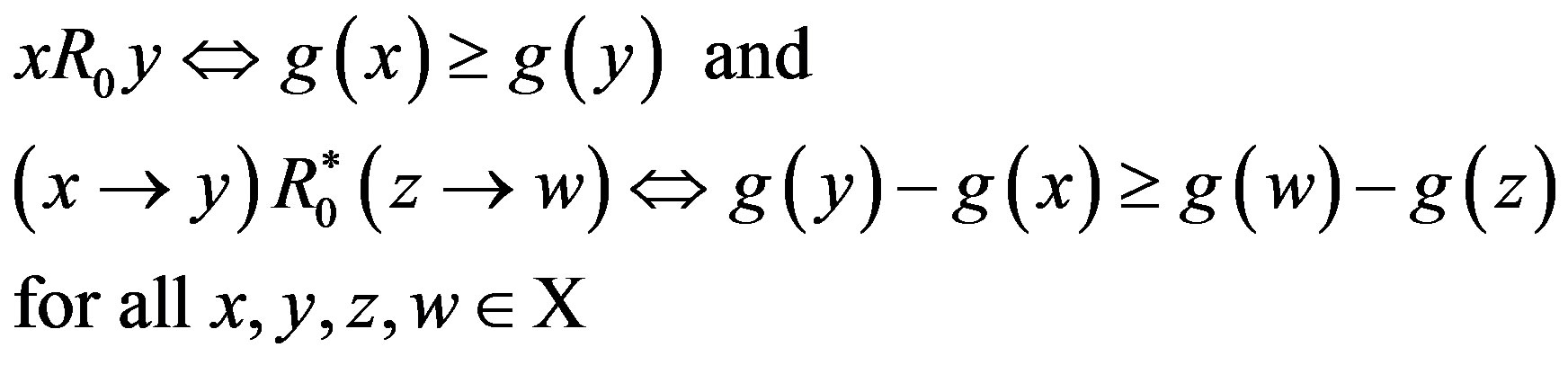
2) for all. This definition implies that, for a given real-valued function u on X, there uniquely exists a preference structure (R, R^*) which is represented by the function u, i.e., if and are represented by u, then. Specifically, let be the preference structure represented by the logarithmic function, i.e.3) for all4) for all. Since the logarithmic function is monotone, the condition 3) means that R₀ is the monotone level comparison relation. 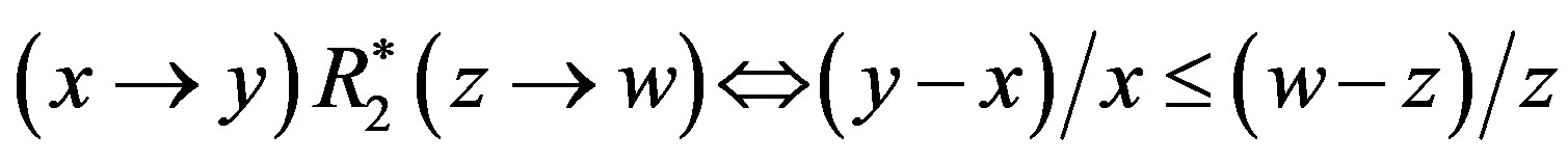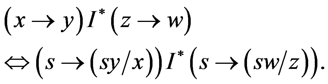For, we need a lemma proved in Appendix B:

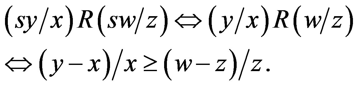
Lemma 1 Û (y/x)R(w/z) Û for all.

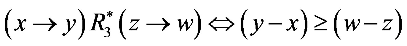
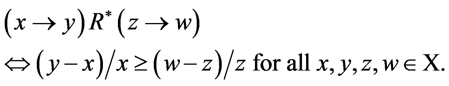
It follows from Lemma 1 that the condition 4) means that the difference comparison relation is determined by the simple rule that the differences with larger growth rates are more desirable, i.e.,

.

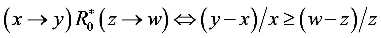2.2. Results

We introduce the following axioms to characterize the representability of a preference structure by the logarithmic function:

Monotonicity for all.

Consistency There exists some such that for all.

Homogeneity for all and all t > 0.

The monotonicity axiom means that the larger levels of income are more desirable, and the consistency axiom means that there exists some such that the difference comparison on and coincides with the level comparison on x and y for all. The homogeneity axiom means that two transitions are indifferent if one transition is given by multiplying a positive number both for the initial and ending levels of another transition. Then we have the following proposition:

Proposition Let (R, R^*) be a preference structure on X and let L be a set of real-valued functions f on X defined by L = {f: there exist a > 0 and b such that for all }. Then the following three statements are mutually equivalent:

1) (R, R^*) satisfies the monotonicity, consistency and homogeneity axioms;

2) (R, R^*) coincides with, i.e., (R, R^*) is represented by the logarithmic function;

3) (R, R^*) is represented by any function in L and no function in L^C represents (R, R^*).

Proposition is proved in Appendix A. The three axioms in the assertion 1) of Proposition are mutually independent, which can be proved by constructing the counter examples: Define a preference structure by

for all. The preference structure satisfies the homogeneity and consistency axioms, but it does not satisfy the monotonicity axiom, which implies that the monotonicity axiom is independent. Let be a difference comparison relation defined by

for all, and let be a difference comparison relation defined by

for all. Letting R₀ be the monotonic level comparison relation again, the preference structure satisfies the monotonicity and homogeneity axioms, but it does not satisfy the consistency axiom, which implies that the consistency axiom is independent. In fact, it holds that 2S₀1 and for all. The preference structure satisfies the monotonicity and consistency axioms, but it does not satisfy the homogeneity axiom, which implies that the homogeneity axiom is independent.

3. Conclusions

A consumer’s preferences over money income levels are specified by a level comparison relation and a difference comparison relation. A pair of the relations is called a preference structure and it is shown that a preference structure is cardinally represented by the logarithmic function if and only if the preference structure satisfies the three mutually independent axioms on the preference structures. This result clarifies the mutually independent axioms characterizing the preference structure represented by the logarithmic function as a cardinal utility function. In particular, this result enables us to interpret the per capita national income measured by the logarithmic scale as the utility level of the income, and axiomatically characterizes the simple rule evaluating the differences of per capita national income levels based on their growth rates under the monotonic level comparison relation.

Funding

The research for this paper is partially supported by Ministry of Education, Science and Culture through JSPS Grant-in-Aids for Scientific Research No. 24530191.

REFERENCES

Appendix A

Proof of Proposition: We can easily show that the assertion 3) implies the assertion 2) and that the assertion 2) implies the assertion 1). First, we show that the assertion 1) implies the assertion 2). Suppose that (R, R^*) satisfies the three axioms. By the contraposition of the monotonicity axiom that

. (1)

Since R is a complete and transitive binary relation on X, it holds that

. (2)

It holds by the monotonicity axiom and (2) that

. (3)

Hence it holds by (1) and (3) that

. (4)

Since is increasing on X, it holds by (4) that

.

Let s be an element in X satisfying the condition in the consistency axiom, i.e.,

. (5)

It holds by the homogeneity axiom that

which implies that

(6)

We have by (5) that

. (7)

Moreover, we have by (4) that 

(8)

Hence it holds by (6), (7) and (8) that

(9)

It holds by (9) and Lemma 1 that

for all. Thus the assertion 2) holds.

Second, we will show that the assertion 2) implies the assertion 3). Suppose that the assertion 2) holds, i.e.,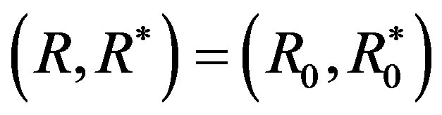. Since the assertion 2) implies the assertion 1), satisfies the three axioms. Moreover, we can easily show that is represented by any function in L. There remains to show that no function in L^C represents. Suppose that a real-valued function g on X represents, i.e., it holds that

(10)

Define a function f: R → R by for all. Then it holds that

. (11)

We need a lemma proved in Appendix B:

Lemma 2: 1)

for all. 2) is continuous and increasing on R.

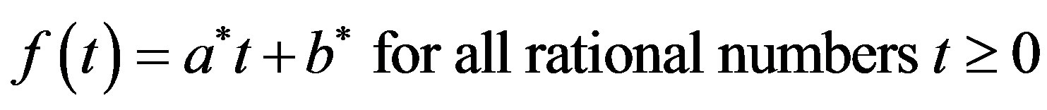
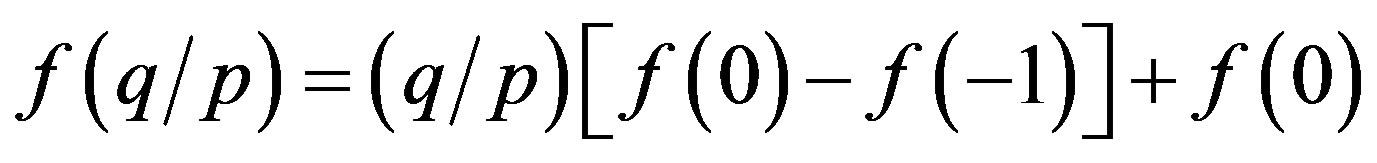
Setting a^* = f(1) − f(0) > 0 and b^* = f(0), we will prove that f(t) = a^*t + b^* for all. Suppose that t is a rational number, i.e., there exists a pair of integers (p, q) such that

. (12)

Using the induction arguments with respect to for a fixed p ≠ 0, it holds by Lemma 2 1) that

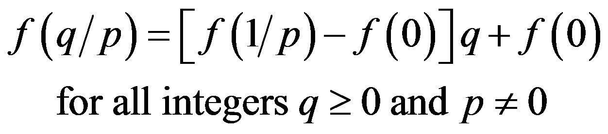(13)

Case 1 (t ≥ 0) Setting q = p in (13), we have that

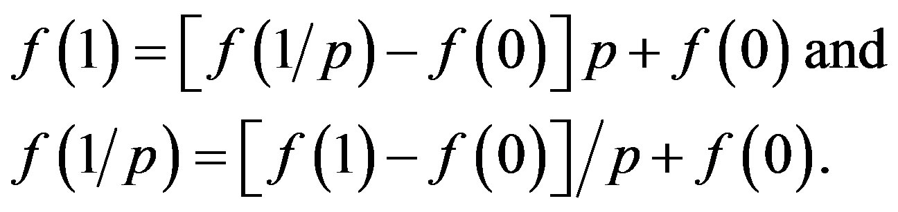
Hence, we have by (13) and this that 

.

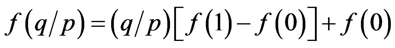Since a^* = f(1) − f(0) and b^* = f(0), we have that

.

Since is continuous on R by Lemma 2 2), we have that

.

Case 2 (t < 0) It holds by (12) that p < 0. Setting q = − p > 0 in (13), we have that

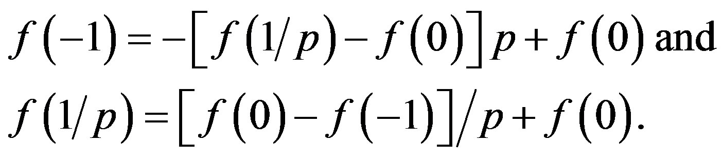
Hence we have by (13) and this that 

.

Since 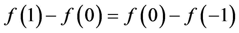by Lemma 2 1), we have that a^* = f(0) − f(−1) > 0. Hence we have that

.

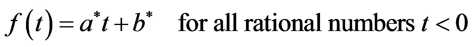Since is continuous on R by Lemma 2 2), we have that

.

Thus it holds by (11) that and that no function in L^C represents.      

Appendix B

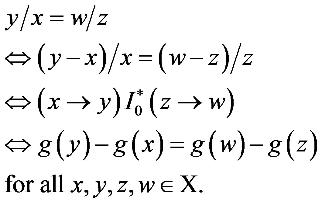
Proof of Lemma 1 It holds that

Û

Û

Û

Û

for all.      

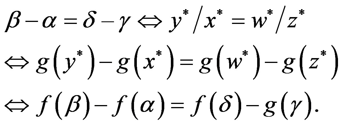
Proof of Lemma 2 1) Since satisfies the three axioms, it holds by Lemma 1 and (10) that

(14)

For any, set x^* = e^α, y^* = e^β, z^* = e^γ and w^* = e^δ. Then we have by (14) that

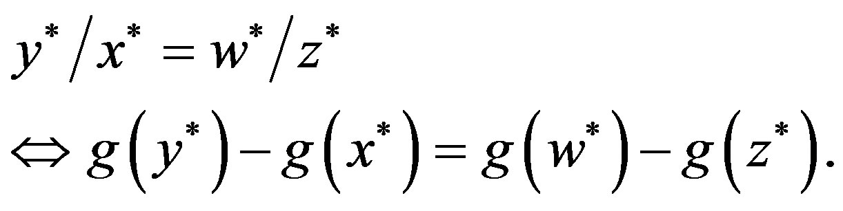
It holds by this and (11) that

2) Since g(x) is (strictly) increasing on X by (10), and since e^t is (strictly) increasing on R, f(t) ≡ g(e^t) is (strictly) increasing on R. Hence it holds by [14] Chapter 5 Theorem 3 p.100 that there are at most countable number of points at which f is not continuous. Thus there is a point α in R at which f is continuous. Let β be a point in R, and let {β_m} be a sequence in R converging to β. Define a sequence {α_m} in R by

.

Hence we have Lemma 2 1) that

.

Since limα_m = α and f is continuous at α, we have that

.      

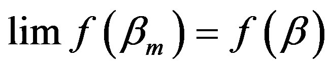NOTES

¹Watts [1] introduces a poverty index, which can be interpreted as the differences of the logarithmic utility values. See [2,3] for the Watts index. For the examples in the growth theory, see [4] Propositions 4 and 5, [5] Chapter 6 Example 6.4, and [6] Appendix Figure A2-2.

²Namely the following three statements for a (rational) level comparison relation R on positive income levels are mutually equivalent: 1) the relation R satisfies the monotonicity axiom, i.e., 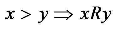and not yRx; 2) the relation R is represented by the logarithmic function, i.e.,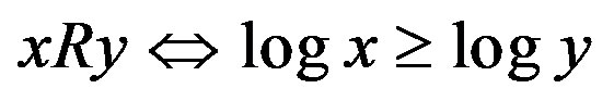; 3) the relation R is represented by any function in M and no function in M^C represents R, where M is the set of all increasing functions on the income levels.

³In the literature of psychophysics, almost the same hypothesis called Weber-Fechner law is assumed for deriving a logarithmic function to represent the relationship between the stimuli and sensations. For the Weber-Fechner law, see [8]. In case of the expected utility function, which is also determined unique up to positive affine transformations, almost the same hypothesis stated in a differential form is assumed by Bernoulli to derive the logarithmic utility function. For the derivation of logarithmic utility function based on Bernoulli hypothesis, see [9] Section 3 and [10] Historical Note 6 Classic logarithmic utility.

⁴For the cardinal utility theory based on the difference comparisons, see [11-13].

REFERENCES

- H. Watts, “An Economic Definition of Poverty,” In: D. P. Moynihan, Ed., On Understanding Poverty, Basic Books, New York, Chapter 11, 1968, pp. 316-329.
- S. R. Chakravarty, “A New Index of Poverty,” Mathematical Social Sciences, Vol. 6, No. 3, 1983, pp. 307-313. http://dx.doi.org/10.1016/0165-4896(83)90064-1
- B. Zheng, “An Axiomatic Characterization of the Watts Poverty Index,” Economics Letters, Vol. 42, No. 1, 1993, pp. 81-88. http://dx.doi.org/10.1016/0165-1765(93)90177-E
- E. Farhi and I. Werning, “Inequality and Social Discounting,” Journal of Political Economy, Vol. 115, No. 3, 2007, pp. 365-402. http://dx.doi.org/10.1086/518741
- D. Acemoglu, “Introduction to Modern Economic Growth,” Princeton University Press, Princeton, 2008.
- O. Blanchard, “Macroeconomics,” 5th Edition, Prentice Hall, Upper Saddle River, 2009.
- P. Suppes, “The Distributive Justice of Income Inequality,” Erkenntnis, Vol. 11, No. 1, 1977, pp. 233-250. http://dx.doi.org/10.1007/BF00169854
- D. J. Murray, “A Perspective for Viewing the History of Psychophysics,” Behavioral and Brain Sciences, Vol. 16, No. 1, 1993, pp. 115-115. http://dx.doi.org/10.1017/S0140525X00029277
- H. Dalton, “The Measurement of the Inequality of Incomes,” Economic Journal, Vol. 30, No. 119, 1920, pp. 348-361. http://dx.doi.org/10.2307/2223525
- P. A. Samuelson, “St. Petersburg Paradoxes: Defanged, Dissected, and Historically Described,” Journal of Economic Literature, Vol. 15, No. 1, 1977, pp. 24-55.
- F. Alt, “Über die Mebarkeit des Nutzens,” Zeitschrift für Nationalökonomie, Vol. 7, No. 2, 1936, pp. 161-169. http://dx.doi.org/10.1007/BF01316465
- L. S. Shapley, “Cardinal Utility Comparisons from Intensity Comparisons,” Report R-1683-PR, The Rand Corporation, Santa Monica, 1975.
- V. Köberling, “Strength of Preference and Cardinal Utility,” Economic Theory, Vol. 27, No. 2, 2006, pp. 375-391. http://dx.doi.org/10.1007/s00199-005-0598-5
- H. L. Royden, “Real Analysis,” 3rd Edition, Macmillan, New York, 1988.