Theoretical Economics Letters
Vol. 3 No. 5A1 (2013) , Article ID: 36259 , 8 pages DOI:10.4236/tel.2013.35A1002
A Consistent Relaxation of the Consumption Invariant Rate in the Discounted-Utility Model
University of Groningen, Groningen, The Netherlands
Email: *mehrajp@live.co.uk
Copyright © 2013 Mehraj Bin Yasaar Parouty et al. This is an open access article distributed under the Creative Commons Attribution License, which permits unrestricted use, distribution, and reproduction in any medium, provided the original work is properly cited.
Received July 22, 2013; revised August 15, 2013; accepted August 20, 2013
Keywords: Matrix Algebra; Discount Rate; Health-Economics
ABSTRACT
The main theoretical contribution of this paper is a mechanical result that relates growth rates across n commodities. We examplify through a 2-commodity economy of health and money where the results of current health economic theory are confirmed using this technology. The applications are, however, broad; both with regards to spacial discount rates by making relevant assumptions about interpersonal/international comparability and to sustainable growth by envisioning scenarios for the future.
1. Introduction
Time preferences are common, important and often lifesaving. Sustainability of factors of production [1], ethical fairness towards future generations [2,3] and cost-effectiveness analyses of preventive programs [4] are a few of the well-known economic debates revolving around different approaches towards valuing of the future. The standard model of intertemporal choice is the discounted utility model (DU-model), which was first introduced by Samuelson [5]. Since then, the axiomatic derivation of the model has been numerous [6-10]. An important assumption of the DU-model is that the discount rate is positive and invariant across time and across all forms of consumptions [11]. However, it is often empirically remarked that individuals do not coordinate their intertemporal preferences with pricing choices [12-15]. Frederick and Loewenstein [13], among others, found that intertemporal preferences generally did not have the expected mapping properties on intertemporal willingnessto-pay. In the health sector, for example, current arguments in Health Technology Assessments (HTAs) concern the theoretical foundation of differential discounting for costs and health outcomes [16,17]. To that end, we relax the assumption of an invariant rate.
We assume a set of n-commodity-specific discount functions and provide a matrix-vector representation of marginal substitutions based on a model consistent expectation. Since we are concerned with marginals, one need not necessarily specify the “absolute” functions, per se, but rather the relative change of a function compared to another. Our model, being valid in cases of negative discount rates as well, derives from a more general concept. Our conceptualisation gained popularity, mostly among physicists, from Einstein’s general theory of relativity in which he considered a set of coordinate system where the metric tensor defined the type of space, flat or curved etcetera. In our case, we note that some function of well-being across time for an n-commodity economy can be geometrically represented by a function of the n-dimensional commodity space where each coordinate changes with time according to some specific functions. With regards to the coordinate transformations, we shall assume that production processes of n different commodities are equivalent to some value-gaining processes such as Rae’s instruments [18], where the value gaining processes are, possibly, dissimilar. Thus a single point can be infinitely characterised by alternative time-dependent coordinate systems. Section 2 provides a theorem of the representation which we prove by induction.
Using arguments such as consistency in intertemporal choices and intercommodity wise, we then have a cyclical representation of marginal valuations. Cyclical mechanisms describing the economy have, for the past few decades, gained the attention of several economists [19,20]. The simplicity of the mathematics of input-output systems has led to extending such systems to open ones as well as to intertemporal ones by adding an additional growth term. An important facet in inputoutput systems generally (if not always) includes some arguments of equivalence relation1. In our case, we firstly equate commodity i’s current input quantities to its future quantity specified by some growth function. Although the quantities of commodities vary stochastically, as a first approach, we propose a model-consistent expectation that assumes that commodities evolve along deterministic (expected) functions of time2. Section 3 provides a visual derivation based on some uniform measure of the commodities or purely on physical quantities of the commodities. Our representation however allows for differential discounting which is a major ethical debate in health economics. As such one might want to investigate the cost-effectiveness with regards to net-monetary gains as well as increased life expectancy or increased standards of life. Section 4 introduces illustrations with such marginal valuations and Section 5 concludes.
2. A Covariance Representation of Coordinate Transformations
Suppose that we have an n-dimensional function, say  described by two sets of coordinate systems, say
  and
and  where the coordinate transformation is given by
  with
with , say. Since a differential,
  , is uniquely characterised in the q0-frame of reference as well as uniquely characterised in the qT-frame of reference, one could consider a differential,
  which can also be characterised by
 . Assuming that we know the set of partial derivatives in the q0-frame of reference,
  , as well as in the qT-frame of reference,
  , we can form a matrix with those known components such that the eigenvector of that matrix, corresponding to an eigenvalue 1, represents the bijective coordinate transformation components,
  , We then have a matrix-vector representation of partial derivatives since we are simply concerned with the derivative of an axis with respect to another (not necessarily orthogonal here).
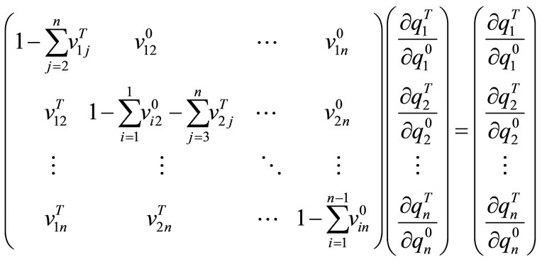
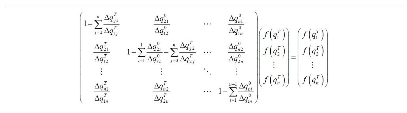
Theorem 2.1. Suppose that we have an n-dimensional space characterized by 2 sets of n-dimensional coordinates, q0 and qT, then, defining  by
by , the matrix
 given by,

has an eigenvalue of 1 that corresponds to the eigenvector3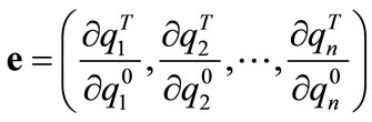 .
.
That is
Proof. Suppose there exists a matrix, X that is non-zero and non-diagonal, given by
such  where
where 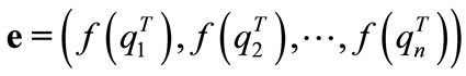 with
with 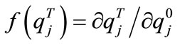
and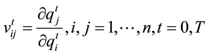 .
.
Then,  satisfies
 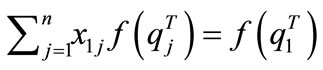 . i.e.
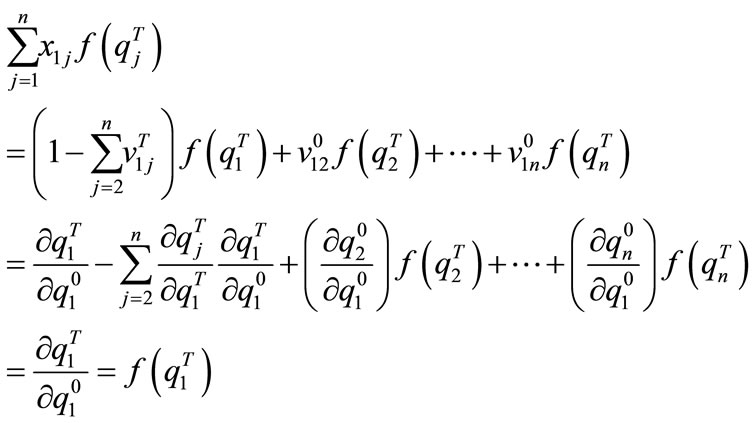
Assume that 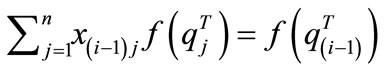 is true.
Then , given by
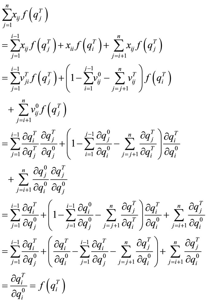
is also true. By induction, X, given by the theorem is deduced.
We now note some properties of the matrix-vector system4 which makes the usage fairly attractive for economists.
1) All the elements of our matrix are partial differentials valued with time being constant (i.e. each components of the matrix are specific to one and only one time point, either t = 0 or t = T).
2) The elements of the vector are partial differentials relating to a single axis (i.e. each of the elements of the vector is specific to one and only one commodity i, i = either 1 or 2 or···or n). Furthermore, the growth vectorsay 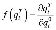 is not specified and the chain rule allows
 to be, say, an exponential growth while
  to be, say, a linear growth, and the general solution of the system of equations is given by:
 (1)
(1)
3. A Derivation with Commodities
Suppose that we have an n-commodity economy where the measures of each commodity evolve through time t, each according to specific growth functions,  ,
, . Without loss of generality, we suppose that the commodity bundle is
 , the n-dimensional Euclidean orthant and the physical quantity of commodity i at time t is denoted
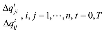
 . Given that we have a closed economy, the ratio of any arbitrary commodity i to another arbitrary commodity j,
  is fully specified at all times. Alternatively, given a system of ratios of all commodities to other commodities at different times, a unique vector of growths exists for each of the n commodities through time. Our quest in this section is to specify a matrix whose entries are the ratios of commodity i to commodity j,
  at specific times, say t = 0 and t = T that would correspond to the growth functions
 .
.
Suppose that we now, time t = 0, have  of commodity i,
  which grows up to time T to
 . We define the growth function,
  to be the ratio of the future quantity of commodity i to its current quantity.
 (2)
(2)
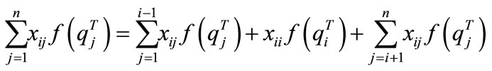
Let  be the quantity of commodity i at time t = 0 that will exchanged for (used in the production of) commodity j, at time t = T. Splitting commodity i into n parts at the present time, we have
 (3)
(3)
where  is the part of commodity i now that will make up for the part commodity j in the future. At that future time, T, the quantity of commodity j,
  ,
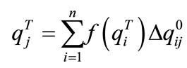
,  , is composed of the total parts from all n commodities, which at time t = 0 were allocated to its future production,
 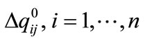 , each forwarded to time T at their respective growth rates,
  . The quantity of commodity j at time t = T is then given by
 (4)
(4)
Now, from Equations (2) and (3), we have
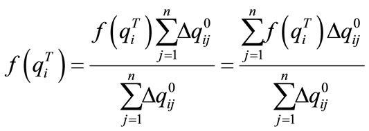 (5)
(5)
and from Equations (2) and (4), we have
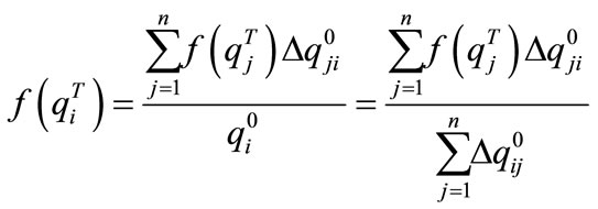 (6)
(6)
Equating Equation (5) with (6),
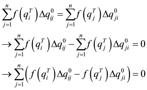
Let us consider the solution  . This solution is the equivalence relation that we shall investigate. In the next section, the continuous version of the equivalence relation,
 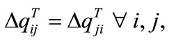 is shown to be a direct conesquence of a major assumption in time preferences, namely the welfare-preserving rate. However, restricting ourselves to physical quantities for the time being, assuming that
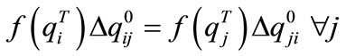 , we have
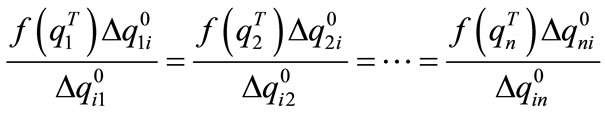
implying that we can write , rather than a ratio of sums, as a sum of ratios5, i.e. Equation (6) becomes
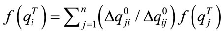 . Thus, with
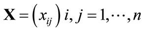
 , we have a system of linear equations which we can write in terms of a matrix of ratiossay
  where
where 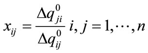
and a vector of growths, say
 such that
 . We shall use the transpose notation to denote column vectors. Further, note that all elements of the Matrix X are ratios valued in the present time only, that is time t = 0.
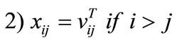
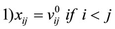
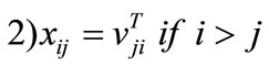
Furthermore, given that we have a closed economy with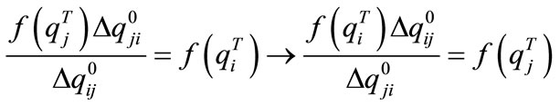 our columns are also specified6. That is, given an entry in the upper triangular matrix, say
 , an entry in the lower triangular matrix, xij , is also specified such that
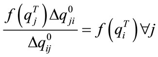
 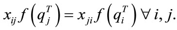 Since it is more of our interest to consider how a single ratio changes, we wish to maintain the numerator and denominator so that they represent the ratio of the same commodities; but at different times. Thus if
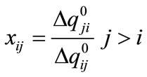 , and remembering that
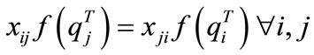 , we let
 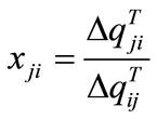 so that it is only the time at which we consithe ratios that is changed7. Next, with
 implying that a unit of commodity j grows to
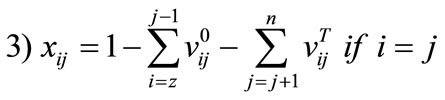
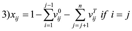
 , we add a further constraint on the diagonal entries. Given that we have
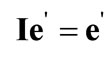 , then we firstly require that
  has an eigenvalue of one corresponding to the eigenvector,
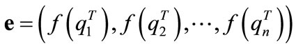 . We thus require that each of the columns of our matrix sum to 1, which is a consequence of equation 3. We therefore condition on the diagonal entries so that xjj equal to
 . Thus we have specified all entries of our matrix of ratios such that
 . That is Without loss of generality, we could consider partial dif-
ferentials rather than ratio of quantities8. Furthermore, such continuity assumptions often allow the incorporation of some economic definitions fairly well. So, we shall let 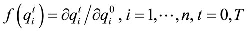 and consequently redefine the terms of our matrix,
 in the traditional partial differential sense. Since the entries of X, only involve the pairwise exchanges,
  i.e. the change in quantity of commodity i at time t that comes from commodity j at time 0 divided by the change in quantity of commodity j at time t that comes from commodity i at time 0, then given that
 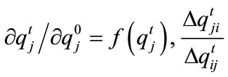 can effectively be stated in a much simpler fashion; i.e. the change in commodity j with respect to commodity i at time t9,
 .
.
Next, suppose we wish to find the matrix inputs at a given time t = T that corresponds to the vector e. Letting  , the partial derivative of commodity j with respect to commodity i at the specific time T, we have the representation theorem.
4. An Illustration in Welfare
The non-specificity of a functional “absolute” form opens doors for the use of the matrix system in various other sectors and for different other purposes. The mathematics of marginal rate of transformation and of marginal rate of substitution, being simply that of marginals or partial differentials, in this subsection, we wish to consider the term “marginal value” as input in our system. In order to justify the matrix approach for marginal substitutions, it is necessary to make various simplifying assumptions: we recall firstly that we have an economy that is closed and is composed of n commodities only; and we further require that our fictitious society satisfies the necessary assumptions required for the existence of an intercommodity and intertemporal indifference curve such as the Von Newman and Morgenstern [21] rationality axioms and the axioms presented by Ok and Masatlioglu [22], for intercommodity and intertemporal conditions respectively.
Definition 4.1. Let the social welfare function, at time t, be  where the commodity bundle is
 , the n-dimensional Euclidean orthant defined before.
Definition 4.2. Let the (negative) marginal substitution for commodity j between its future quantity and its current quantity be denoted as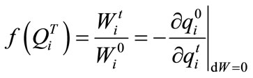 where
where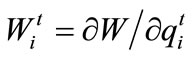 .
.
Definition 4.3. We further denote the (negative) social marginal rate of substitution between commodity j and commodity i at time , as,
, as, 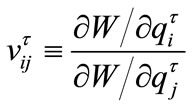
Remarks. Definition 4.3, having a bijective nature, should remind us of the equivalence relation from the previous section;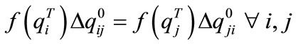 . However, in order to use the representation for preferences, we shall require an independence condition introduced by Leontief [23]. To do so, we impose the equivalence lemma of Stigum [24]:
Definition 4.4. Let  be a partition of the set of variables, K, and let
  be any set of non-negative quantities of the variables in
 . The group of variables,
  is separable in W from a variable Kk, if and only if the correspondence, β, defined by
 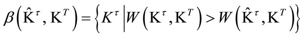 , is independent of qk, the quantity of the variable Kk.
Remarks. This definition is equivalent to the condition that the marginal rates of substitution at time ,
,
 , is independent of
  [25]. If
  is twice differentiable, then the condition is equivalent to
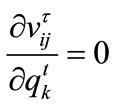 .
.
Since we again have two sets of partial differentials where each set, in turn, relate to each other through partial differentials10, we can write, with such definitions,
where xij is defined as in theorem 2.1. and we have a consistent representation of marginal substitutions. Although the above definitions assume the welfare preserving rate, with other welfare models, adjustments for dw can be made ex-ante since our representation builds on the basis differential, dq.
A Representation for Health Economists
Although there have been several debates in literature regarding differential time preferences, we focus on discounting of health outcomes in this subsection and validate our representation with current health-economic literature. While education, for example, is commonly known, with several empirical evidences, to boost both health and income, other economic activities are known, on the one hand, to be favourable to economic growth, while, on the other hand, to impact negatively on the population’s health. As Myrdal stated, production is a circular and cumulative sequence of causations [26]. Historians such as [27], for example, also noted that “all forms of economic growth exert intrinsically negative population health effects among the communities that are most directly involved in the transformations which they entail”.
Consequently, in order to represent current health economic discounting with our system, we shall restrict ourselves to a 2-commodity economy; namely income and the QALY, a unique measure of health outcome which is the combination of quality of life and life years. To restricting ourselves, again, to welfare preserving rates for money and health, In order to illustrate our matrix approach, we let commodity 1 and 2 be health, h, and money, m, respectively and use a one year time period,  , for this illustration. Let our social welfare function be summarised over only money streams and health streams, say
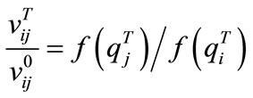
 . Letting the marginal value of future money in terms of current money be denoted by
 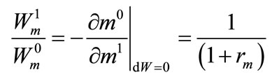 and let the marginal value of future health in terms of current health be denoted by
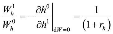 , we denote the
(negative) social marginal rate of substitution between money and health by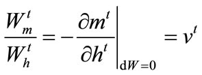 ;
;
where 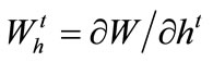 is the marginal social welfare from an infinitesimal increase in health at time t and
 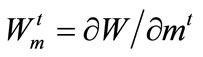 is the marginal social welfare from an infinitesimal increase in money at time t. From above theorem, in the case n = 2, we get the following system:
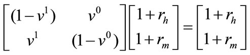
with solution,
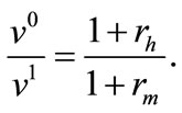 (7)
(7)
that is, “The marginal value of one good (health or income) in terms of another is the same whatever the route by which they are compared”, as gravelle stated. By considering the NPV of an intervention from two equivalent ways, Gravelle and Smith showed in a very straight forward way that v0 and v1 are related in the same linear fashion as above. They considered a single one year period11 example where an intervention changes present and future costs by  and
and  respectively and the quantities of present and future health by
  and
and  respectively. Firstly, they valued health effects in each period in terms of income and then discounted the future value at the rate of interest on income, rm. Secondly, they converted the change in future health into an equivalent change in current health and then applied the value of current health in terms of current income. Then, by their consistency argument, equating the two NPV’s yields Equation (7).
The reason why the matrix method is similar to the NPV method is that they are both solutions to the same problem. The aim was to find a relationship between v0 and v1 with the given constraints that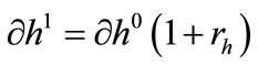 ,
,
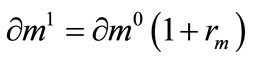 , and
, and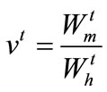 . Thus in order to be indifferent to the gain of (1 + rh) of future health at time t = 1, consistency requires that we could now, at time zerohold either 1 unit of health only or
  units of income only or, in our case, we hold both income and health in the proportions: (1 − v1) units of health and v0 units of wealth. We see that, in the example given by Gravelle and Smith, in order to have
  of health at time t = 1, they either hold
 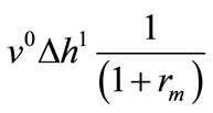 of health now or
 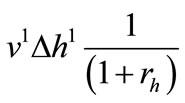 of income now. Thus, our 2 × 2 matrix and the NPV approaches provide the same results.
5. Discussion
Our approach resembles, to some degree, that of the original cyclical mechanisms that were proposed by Quesnay Tableau economique [28]. We, however, rather than equating the “physical quantity on the side of the means of production to that on the side of the product, both of which consist of the same product” [20], allow for a non-fixed timing of the production process similar to Rae’s instruments, which we equate through Euclid’s proposition 12. It might not be unimportant to note that, while this paper addresses consistency in preferences, using growths in physical quantities of a single product, investigations on a sustainable production-consumption cycle seem fairly attractive. Alternatively, plugging in rates of time preferences as growth parameters of different commodities might aid in investigating consistency among social discount rates.
As Riccardo’s methodology in devising rates of profits of a farmer by singling out corn as a ‘basic’ commodity, we choose to, rather, single out health measures as basic commodity. Analogous to Riccardo’s conclusion with that regards, we propose that “it is the growth in health that regulate the growth in other trades/commodities”. As a generic measure for health, the quality-adjusted life year (QALY) is often used. While the QALY is a multiplicative combination of health quality and life duration which is also consistent with health states that are worse than death or have zero duration of life, the assumption of linear utility of duration is often weakened for simplicity and challenges the actual discounting of the generic concept. We therefore suggest that the QALY be treated as its two different constituents, namely quality of life and the life years; which also strengthens the idea of an array-cost-effectiveness analysis. As such, our representation theorem opens the route to formally investigate potentially different discount rates for quality of life and life years which could especially be important for evaluating cost-effectiveness of life saving and life improving medical interventions differently.
REFERENCES
- P. Dasgupta, K. G. Maler and S. Barrett, “Intergenerational Equity, Social Discount Rates and Global Warming,” In: P. R. Portney and J. P. Weyant, Eds., Discounting and Intergenerational Equity, Johns Hopkins University Press, Baltimore, 2000, pp. 51-77.
- A. C. Pigou, “The Economics of Welfare,” Macmillan, London, 1920.
- J. Rawls, “A Theory of Justice,” Clarendon Press, Oxford, 1972.
- J. M. Bos, M. J. Postma and L. Annemans, “Discounting Health Effects in Pharmacoeconomic Evaluations: Current Controversies,” Pharmacoeconomics, Vol. 23, No. 7, 2005, pp. 639-649. doi:10.2165/00019053-200523070-00001
- P. Samuelson, “A Note on Measurement of Utility,” Review of Economic Studies, Vol. 4, No. 2, 1937, pp. 155- 161. doi:10.2307/2967612
- P. C. Fishburn, “Utility Theory and Decision Making,” Wiley, New York, 1970.
- T. C. Koopmans, “Stationary Ordinary Utility and Impatience,” Econometrica, Vol. 28, No. 2, 1960, pp. 287-309. doi:10.2307/1907722
- K. J. Lancaster, “An Axiomatic Theory of Consumer Time Preference,” International Economic Review, Vol. 4, No. 2, 1963, pp. 221-231. doi:10.2307/2525488
- R. F. Meyer, “Preferences over Time in Decisions with Mulltiple Objectives,” In: R. Keeney and H. Raiffa, Eds., Decisions with Multiple Objectives by Keeney and Raiffa, Chapter 9, Wiley, New York, 1976, pp. 473-489.
- A. Rubinstein, “Is It Economics and Psychology? The Case of Hyperbolic Discounting,” 2000.
- S. Frederick, G. Loewenstein and T. O’Donoghue, “Time Discounting and Time Preference: A Critical Review,” American Economic Association, Vol. 40, No. 2, 2002, pp. 351-401.
- O. Amir and D. Ariely, “Decisions by Rules: The Case of Unwillingness to Pay for Beneficial Delays,” Journal of Marketing Research, Vol. 44, No. 1, 2007, pp. 142-152. doi:10.1509/jmkr.44.1.142
- S. Frederick and G. Lowenstein, “Conflicting Motives in Evaluations of Sequences,” Journal of Risk and Uncertainty, Vol. 37, No. 2, 2008, pp. 221-235. doi:10.1007/s11166-008-9051-z
- D. Kahneman and C. Varey, “Notes on the psychology of utility,” In: J. Roemer and J. Elster, Eds., Interpersonal Comparisons of Well-Being, Cambridge University Press, Cambridge, 1991, pp. 127-159. doi:10.1017/CBO9781139172387.006
- G. Loewenstein and D. Prelec, “Preferences for Sequences of Outcomes,” Psychological Review, Vol. 100, No. 1, 1993, pp. 91-108. doi:10.1037/0033-295X.100.1.91
- H. Gravelle and D. Smith, “Discounting for Health Effects in Cost-Benefit and Cost-Effectiveness Analysis,” Health Economics, Vol. 10, No. 7, 2001, pp. 587-599. doi:10.1002/hec.618
- E. B. Keeler and S. Cretin, “Discounting of Life-Saving and Other Non-Monetary Effects,” Management Science, Vol. 29, No. 3, 1983, pp. 300-306. doi:10.1287/mnsc.29.3.300
- J. Rae “The Sociological Theory of Capital,” Macmillan, London, 1834.
- W. Leontief, “Input-Output Economics,” 2nd Edition, Oxford University Press, New York, 1986.
- P. Sraffa, “Production of Commodities by Means of Commodities: Prelude to a Critique of Economic Theory,” Cambridge University Press, Cambridge, 1960.
- J. V. Neumann and O. Morgenstern, “Theory of Games and Economic Behavior,” 3rd Edition, Princeton University Press, Princeton, 1953.
- E. Ok and Y. Masatlioglu, “A General Theory of Time Preferences,” New York University, New York, 2003.
- W. Leontief, “Introduction to a Theory of Internal Structure of Functional Relationships,” Econometrica, Vol. 15, No. 4, 1947, pp. 361-373. doi:10.2307/1905335
- B. P. Stigum, “On Certain Problems of Aggregation,” International Economic Review, Vol. 8, 1967, pp. 349-367.
- C. Blackorby, D. Nissen, D. Primont and R. R. Russel, “Consistent Intertemporal Decision Making,” The Review of Economic Studies, Vol. 40, No. 2, 1973, pp. 239-248. doi:10.2307/2296650
- G. Myrdal, “Economic Theory and Underdeveloped Regions,” Methuen & Co., Ltd., London, 1963.
- S. Szreter, “Industrialisation and Health,” British Medical Bulletin, Vol. 69, No. 1, 2004, pp. 75-86. doi:10.1093/bmb/ldh005
- F. Quesnay, “Quesnay’s Tableau Economique,” 1759.
NOTES
*Corresponding author.
1For example, Sraffa’s system equates the value (price times quantity) of a product of each industry to the value of all goods and services absorbed by this same industry.
2Throughout this paper, subscripts shall denote commodities and superscripts shall denote time.
3The vector might, as well, be representative of scalars, such as a tensor of rank 0.
4Note that the theorem is consistent with Cramer’s rule.
5This follows from Euclid’s proposition 12, The Elements, Book V. That is: “If any number of magnitudes be proportional, as one of the antecedents is to one of the consequents, so will all the antecedents be to all the consequents”.
6Analogous to Sraffa’s note relating to a system in a self-replacing state (page 5 of the production of commodity by means of commodity), our formulation presupposes a system undergoing indefinite growth. As a result such a state is feasible merely by changing the ratios in which the individual equations enter it.
7To maintain numerator and denominator of  and
and , note that
  can be achieved by forwarding the numerator of the time zero ratio or by discounting the denominator of the time t ratio, i.e.
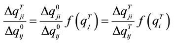 .
.
8For example 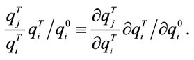
9The use of partial differentials in the system provides a broader set of possibilities of definitions. However, restricting ourselves to the purpose of this paper, we treat the usage as being a continuity of proportional change.
10It is necessary for the chain-rule to hold.
11Gravelle and Smith considered a period of time t = 0 and a period of time t = 1 and the definition they used was two-period while we use specific times t = 0 and t = 1 and hence assume a single period. The derivation however follows.