Theoretical Economics Letters
Vol. 3 No. 1 (2013) , Article ID: 28136 , 5 pages DOI:10.4236/tel.2013.31002
Modeling a Married Couple’s Reciprocal Relationship
School of Business and Economics, Indiana University-Northwest, Gary, USA
Email: tinlin@iun.edu
Received December 2, 2012; revised January 3, 2013; accepted February 5, 2013
Keywords: Reciprocal Relationship; Static Games of Complete Information; Nash Equilibrium; Married Couple
ABSTRACT
A model was developed and a static game of complete information was applied in an examination of a married couple’s reciprocal relationship. Each chose best strategies (i.e., optimal responses) to maximize payoffs (i.e., happiness). Theoretical analysis suggests that the couple’s happiness is endogenously and positively correlated and simultaneously determined. If the wife (or the husband) is not happy with the relationship, it is impossible for the husband (or the wife) to be happy with the relationship.
1. Introduction
The economics literature is replete with studies relating to marriage. For example, Becker’s altruist model (1974 [1], 1991 [2]) looked at how resources are distributed within the family. The bargaining models found in cooperative game theory investigate how husband and wife bargain for a final allocation, with an outside threat point provided by divorce (e.g., Manser and Brown, 1980 [3]; McElroy and Horney, 1981 [4]; McElroy, 1990 [5]; Lundberg and Pollak, 1993 [6]). The threat point in the separate spheres bargaining model of Lundberg and Pollak (1993) [6] is internal to the marriage rather than external, as in the divorce-threat bargaining models (Manser and Brown, 1980 [3]; McElroy and Horney, 1981 [4]). The non-cooperative models examine how each spouse voluntarily provides household public goods, choosing actions that are utility-maximizing given the actions of their partner, and the two settle on a Nash equilibrium (e.g., Lundberg and Pollak, 1994 [7]). Recently, the two-stage models were used to investigate a couple’s decision that affects future bargaining power. For example, Lundberg and Pollak (2003) [8] analyze the two-earner-couple location game. The first stage determines whether the couple remains together, while the second stage determines their location within the marriage. Pollak (2005) [9] argues that wage rates, not earnings, determines bargaining power in marriage. Therefore, in a bargaining model with household production, the main source of bargaining power in marriage is a spouse’s productivity in home production.
In this paper, we adopt an alternative approach and focus on a different perspective by applying a static game of complete information to analyze how a married couple builds a reciprocal relationship and to determine the Nash equilibrium..
2. The Reciprocal Relationship Model
Consider a married couple who are economic individuals and wish to have a successful marriage. Success depends on how each spouse develops their reciprocal relationship. Without a wife, a husband cannot independently produce a reciprocal relationship. Similarly, without a husband, a wife also cannot independently produce a reciprocal relationship. Thus, the reciprocal relationship must be produced by both the husband (denoted as h) and the wife (denoted as w) jointly and simultaneously. Further, it is primarily based on the husband’s response to his wife (denoted ) and the wife’s response to her husband (denoted
 ). Assuming that both responses (
 and
and ) can be quantified as a numerical scale
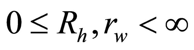 . The higher scale of
  or
or  indicates a more loving response from one to the other, and vice versa. The worst response is scaled as 0, which means that the response can destroy the relationship completely.
We assume that the output function of the reciprocal relationship,  , may be displayed in the Cobb-Douglas form:
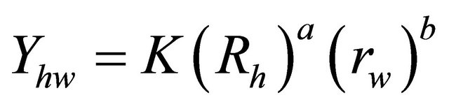 , (1)
, (1)
where  are exogenous variables that consist of several exogenous variables (e.g., maturity, personality, communication skill, hobbies, temper, religious/political beliefs, emotional quotient, compromise ability, financial ability, and unexpected factors); and
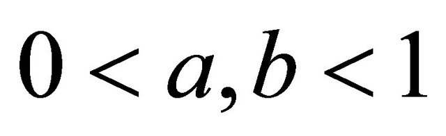 , and
, and  (so that the first-order condition can be sufficient for a maximum effect). In addition,
  and
and  are constant parameters and shares of the husband’s response to his wife (i.e.,
 ) and the wife’s response to her husband (i.e.,
 ) in this relationship output function, respectively. Note that the share of one’s response to the other indeed is the response elasticity of relationship demand. Further, the Cobb-Douglas form is used because the reciprocal relationship is produced by both the husband and the wife jointly and simultaneously. If either one offers a worst response (i.e.,
  or
or ), the relationship output will be zero, implying that the marriage will be completely destroyed. The CobbDouglas form satisfies the assumption, so it is the most appropriate form for displaying the reciprocal relationship. The CES and linear forms cannot satisfy the assumption. Thereby, the Cobb-Douglas form is selected.
Additionally, both have expectation costs of responses. When the one lovingly responds to the other, one would expect an equally nice or better response from the other. If not, one may become frustrated. Thus, as long as there is an expectation, there is a cost from the expectation. The higher the expectation is, the higher the cost is. Therefore, the husband’s expectation cost of response  is illustrated as below:
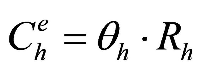 , (2)
, (2)
where 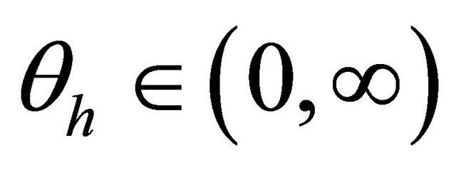 is the husband’s marginal cost of response. Meanwhile, the wife’s expectation cost of response
  is written as:
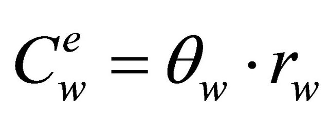 , (3)
, (3)
where 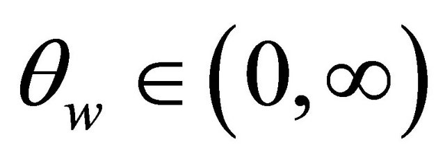 is the wife’s marginal cost of response. A higher marginal cost of response implies that the person may be more sensitive to responses and hence has higher expectations.
Moreover, each one has his/her own payoff from producing the relationship. The husband’s payoff  is specified as below:
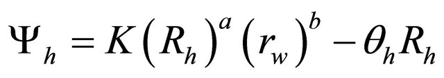 , (4)
, (4)
The wife’s payoff 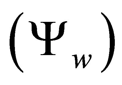 is illustrated as below:
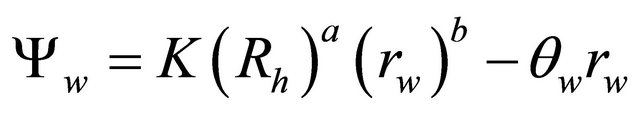 , (5)
, (5)
The payoffs are not monetary. Rather, they indicate a person’s happiness and/or well-being (i.e., utility). The relationship output , shown in Equation (1), is produced both jointly and simultaneously, so their output functions must be the same. Hence, expectation costs are the only difference between their payoff functions.
3. The Nash Equilibrium
Both the husband and the wife are economic individuals and thus seek to receive their best payoffs. Therefore, both will play the game and choose their best strategies in order to receive their best payoffs. The husband seeks great “happiness” from his wife by producing the relationship. The wife also seeks great “happiness” from her husband by producing the relationship. Both players simultaneously choose actions. In other words, this game may be viewed as a static game of complete information (i.e., a simultaneous-move game).
In the game, both players choose their best strategies, which are their responses (i.e.,  and
and ). In the model, the strategies available to each player are their individual responses. As we assumed earlier, response may be quantified according to a numerical scale; thus, the numerical scale is continuously divisible and the negative scale is not feasible. Hence, each player’s strategy space is identified as
 , the nonnegative real numbers, in which a typical strategy s is a numerical scale choice of response,
 . However, we assume that an extremely large numerical scale of response (i.e.,
![]() ) is not feasible because any normal person’s feasible numerical scale of response is limited. Thus, we assume that
) is not feasible because any normal person’s feasible numerical scale of response is limited. Thus, we assume that  and
and 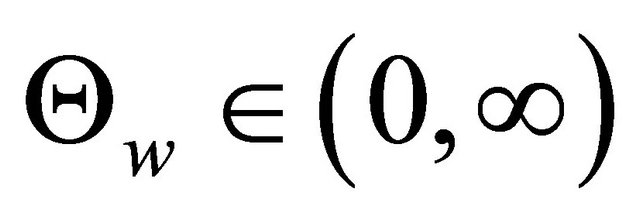 are the maximum number of feasible numerical scales of response for the husband and the wife, respectively (i.e.,
 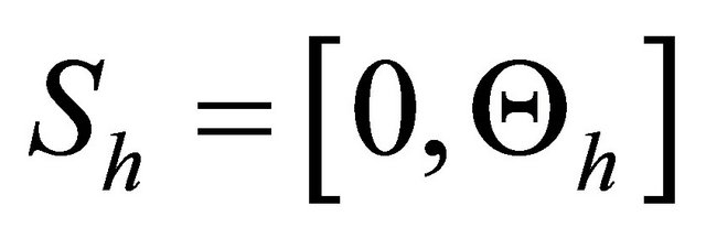 and
and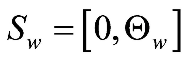 ).
).
Definition 1:
In a two-player game in a normal form, the strategy pair 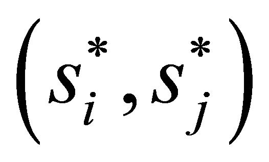 is a Nash equilibrium if, for each player i,
 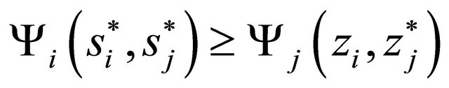 for every feasible strategy
 ![]()
in . For each player i,
  must solve the optimization problem:
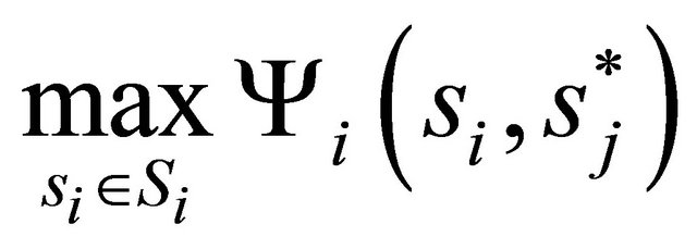 .
.
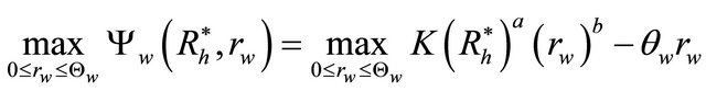
In the model, the numerical scale of response pair  is a Nash equilibrium if, for the husband,
  solves:
 .
.
The first-order condition for the husband’s optimization problem is both necessary and sufficient; it yields:
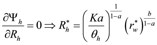 . (6)
. (6)
Similarly, for the wife,  solves:
 .
.
The first-order condition for the wife’s optimization problem is also both necessary and sufficient; it yields:
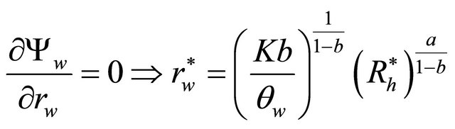 . (7)
. (7)
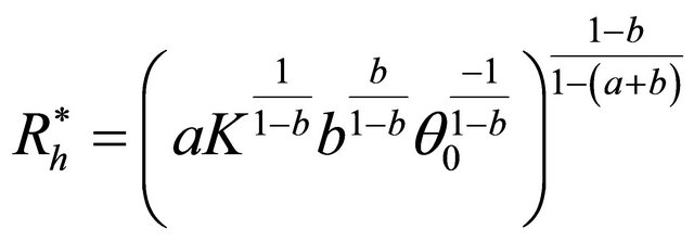
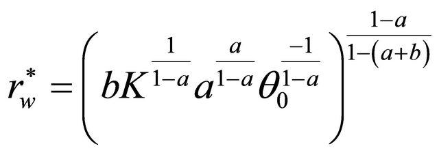
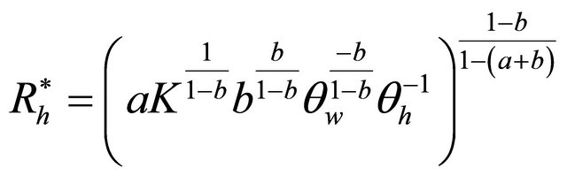
If the numerical scale of response pair  is to be a Nash equilibrium, the players’ response choices must satisfy both Equations (6) and (7). To solve Equations (6) and (7), substituting Equation (7) into Equation (6) yields Equation (8), and substituting Equation (8) into Equation (7) yields Equation (9). Hence, they are:
 (8)
(8)
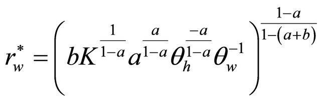 (9)
(9)
The numerical scale of response pair  is the Nash equilibrium; and
 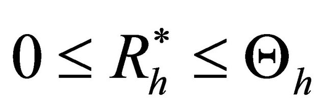 and
and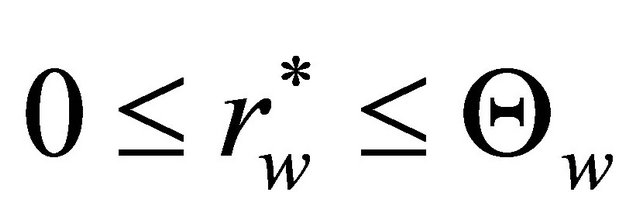 .
.
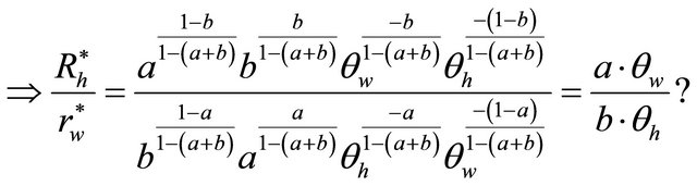
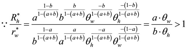
As shown in Equations (8) and (9), 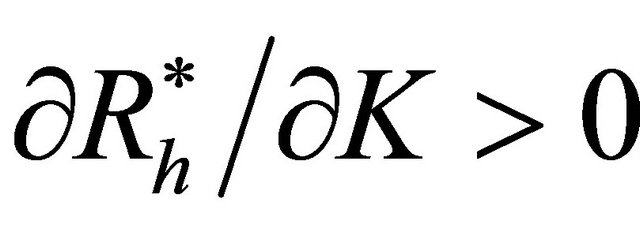 ,
,
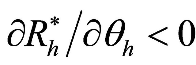 ,
, 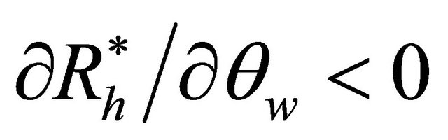 ,
, 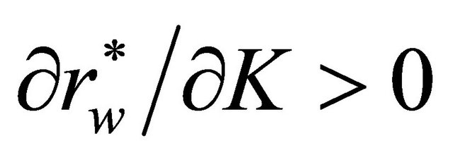 ,
, 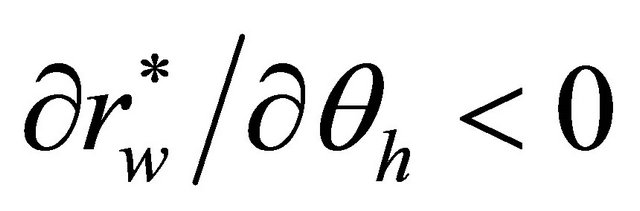 , and
, and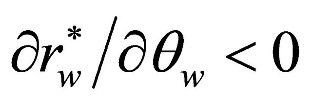 .
.
Proposition 1:
If the shares of both players’ responses are equal (i.e., ) and their marginal costs of responses are also equal
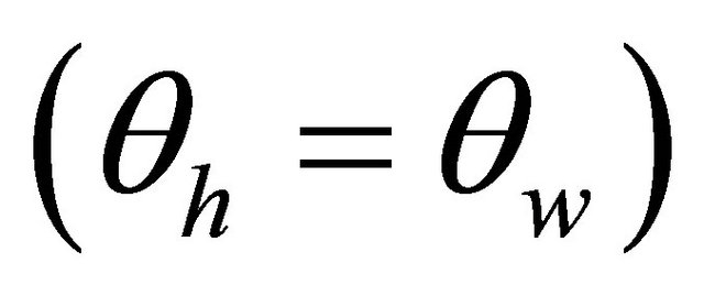 , then both players will offer the same optimal numerical scales of responses to produce the reciprocal relationship.
Proof:
As shown in Equations (8) and (9), if  and
and , obviously, Equation (8) will be equal to Equation (9); that is,
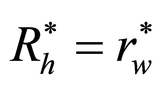 . Q.E.D.
Proposition 1 implies that if both the husband’s and the wife’s response elasticity of relationship demand is equal and both are the same sensitive to responses, then both would offer the same loving responses to produce the relationship.
Proposition 2:
Given the same shares of both players’ responses (i.e., ), if the one’s marginal cost of response is higher than the spouse’s marginal cost of response (i.e.,
  or
or ), then the one will offer a lower optimal numerical scale of response than the spouse’s to produce the reciprocal relationship, vice versa.
Proof:
If  and
and , then
and
 .
.
(Because  and
and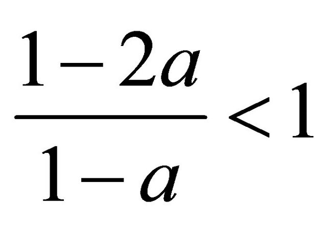 ).
).
 . Similarly, we can show that if
  and
and , then
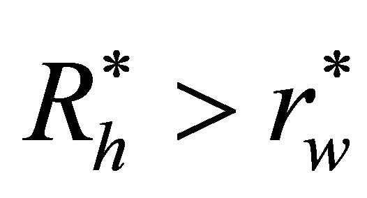 . Q.E.D.
Proposition 2 implies that even though both have the same response elasticity of relationship demand, if the husband is more sensitive to responses than his wife, the husband would offer relatively less loving response than his wife’s to produce the relationship in order to lower his expectation cost, vice versa.
Proposition 3:
Given the same marginal costs of both players’ responses (i.e., ), if the one’s share of response is higher than the spouse’s share of numerical scale of response (i.e.,
  or
or ), then the one will offer a higher optimal numerical scale of response than the spouse’s to produce the reciprocal relationship, vice versa.
Proof:
If  and
and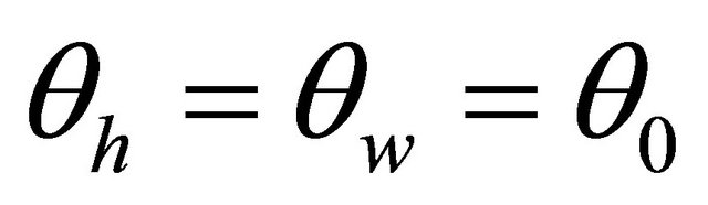 , then
and
 (Because
 )
)
 . Similarly, we can show that if
  and
and , then
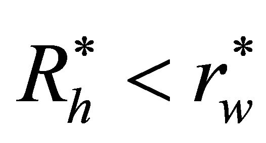 . Q.E.D.
Note that if both the husband and the wife increase one percentage numerical scale in response at the same time, the husband will make a greater percentage increase in the relationship than the wife. This means that the husband would play a more important role than the wife in the process of producing the relationship. For that reason, Proposition 3 indicatesthat if the husband’s relationship demand is more elastic than the wife’s, the husband would likely want to take on more responsibilities in the process. Therefore, the husband will offer more loving response than the wife’s in producing the relationship, vice versa.
Proposition 4:
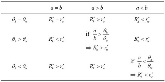
If one’s share and marginal cost of responses are higher than the spouse’s (i.e., 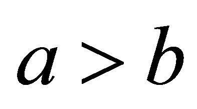 ,
,  or
or ,
, ) then one will offer a greater optimal numerical scale of response than will the spouse in producing the reciprocal relationship only if the ratio of both players’ shares of responses are higher than the ratio of both players’ marginal costs of responses (i.e.,
 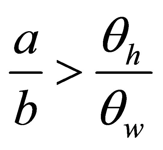 or
or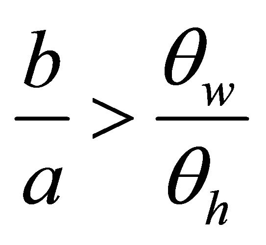 ), vice versa.
Proof:
If  and
and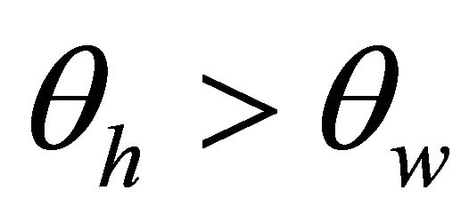 , then
and

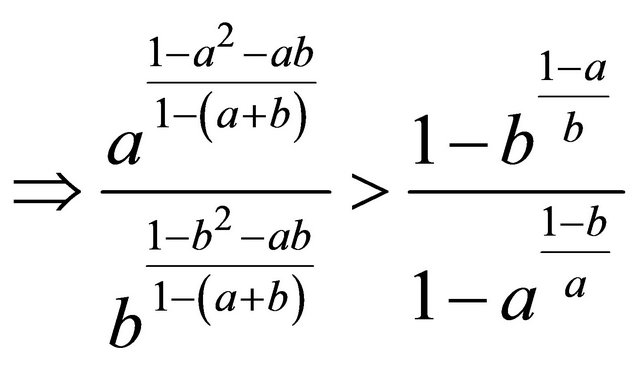
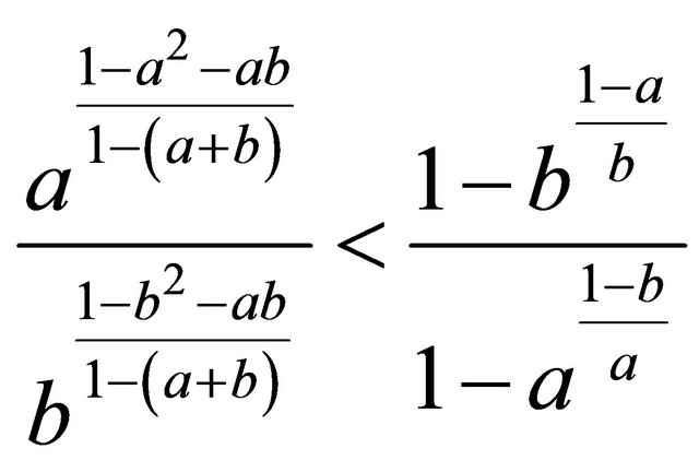
If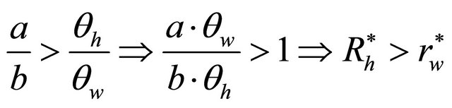 ; orif
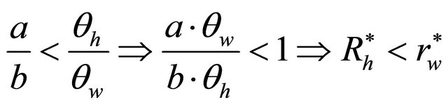 . Q.E.D.
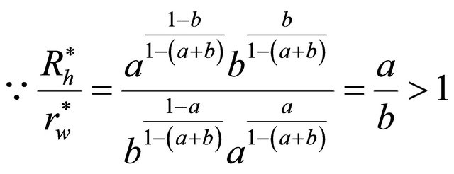
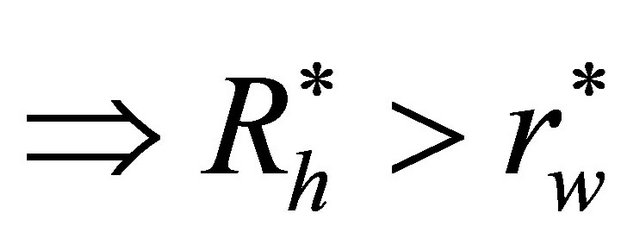
Proposition 4 shows that if the husband’s relationship demand is more elastic than his wife’s and he is also more sensitive to responses than his wife, the only way in which the husband can offer more loving response than his wife is when the ratio of both the husband’s and the wife’s response elasticity of relationship demand is higher than the ratio of their marginal costs of responses.
Proposition 5:
If one’s share of response is larger than the spouse’s while one’s marginal cost of response is lower than the spouse’s (i.e.,  ,
,  or
or ,
,  ,) then one will offer a greater optimal numerical scale of response than the spouse in producing the reciprocal relationship, vice versa.
Proof:
If  and
and , then

and

 .
.
 . Similarly, we can show that if
 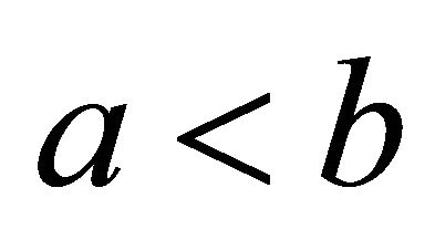 and
and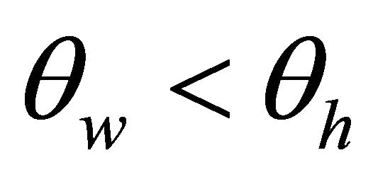 , then
 . Q.E.D.
Proposition 5 indicates that if the husband’s relationship demand is more elastic than his wife’s while he is relatively less sensitive to responses than his wife, the husband would be more likely to offer more loving response in producing the relationship, vice versa.
Propositions 1 - 5 can be summarized as follows.
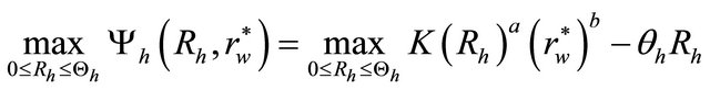
4. The Payoffs
To compute both players’ payoffs, we substitute Equations (8) and (9) into Equations (4) and (5), which yields  and
and , which are the husband’s and the wife’s payoffs, respectively. They are shown as below:
 (10)
(10)
 (11)
(11)
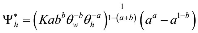
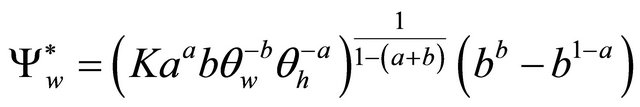
Proposition 6:
Both players’ payoffs are nonnegative. In addition, even if both players’ marginal costs of responses differ (i.e., ), as long as their shares of responses are equal
 , both players will receive the same payoffs (i.e., happiness).
Proof:
As shown in Equations (10) and (11), 
 and
and ,
,  and
and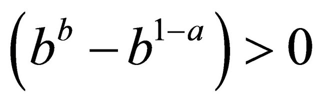 . In addition, K,
  , and
, and  are all nonnegative; therefore,
  and
and ; both players’ payoffs are nonnegative. Moreover, if
 , obviously, Equation (10) will be equal to Equation (11); that is,
 . Q.E.D.
Proposition 7:
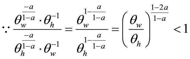
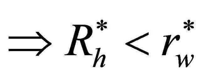
If both players’ shares of responses are different (i.e.,  or
or ), the husband receives a higher payoff than the wife does only if
 . On the other hand, the wife receives a higher payoff than the husband does only if
 .
.
Proof:
As shown in Equations (10) and (11), if the husband’s payoff is higher than the wife’s payoff (i.e., ), then
 .
.
Similarly, we can show that if , then
 . Q.E.D.
5. Conclusion
In this paper we developed a model and applied a static game of complete information to analyze a married couple’s reciprocal relationship. Both the husband and the wife wish to have a successful marriage so they choose their best strategies (i.e., optimal responses) to maximize their payoffs (i.e., happiness). Based upon the premise that both the husband and the wife are economic individuals, the theoretical analysis suggests that the husband’s and the wife’s happiness are endogenously and positively correlated and simultaneously determined. That is, if the wife (or the husband) is not happy with the relationship, it is impossible for the husband (or the wife) to be happy with the relationship, vice versa.
6. Acknowledgements
I would like to thank the anonymous referee and discussants at the ASSA meeting for very helpful discussion and advice.
REFERENCES
- G. Becker, “A Theory of Social Interactions,” Journal of Political Economy, Vol. 82, No. 6, 1974, pp. 1063-1094. doi:10.1086/260265
- G. Becker, “A Treatise on the Family,” Enlarged Edition, Harvard University Press, Cambridge, 1991.
- M. Manser and M. Brown, “Marriage and Household Decision-Making: A Bargaining Analysis,” International Economic Review, Vol. 21, No. 1, 1980, pp. 31-44. doi:10.2307/2526238
- M. McElroy and M. Horney, “Nash-Bargained Household Decisions: Toward a Generalization of the Theory of Demand,” International Economic Review, Vol. 22, No. 2, 1981, pp. 333-349. doi:10.2307/2526280
- M. McElroy, “The Empirical Content of Nash-Bargained Household Behavior,” Journal of Human Resources, Vol. 25, No. 4, 1990, pp. 559-583. doi:10.2307/145667
- S. Lundberg and R. Pollak, “Separate Spheres Bargaining and the Marriage Market,” Journal of Political Economy, Vol. 101, No. 6, 1993, pp. 988-1010. doi:10.1086/261912
- S. Lundberg and R. Pollak, “Noncooperative Bargaining Models of Marriage,” American Economic Review, Vol. 84, No. 2, 1994, pp. 132-137.
- S. Lundberg and R. Pollak, “Efficiency in Marriage,” Review of Economics of the Household, Vol. 1, No. 3, 2003, pp. 153-168. doi:10.1023/A:1025041316091
- R. Pollak, “Bargaining Power in Marriage: Earning, Wage Rates and Household Production,” NBER Working Paper No. 11239, 2005.