Theoretical Economics Letters
Vol. 2 No. 5 (2012) , Article ID: 25537 , 8 pages DOI:10.4236/tel.2012.25078
The Effects of Opening Trade on Regional Inequality in a Model of Scale-Invariant Growth and Foot-Loose Capital
1Graduate School of Economics, Kobe University, Kobe, Japan 2Department of Economics, University of Florida, Gainesville, USA
Email: 2katsufumi.fukuda@gmail.com
Received July 27, 2012; revised August 29, 2012; accepted September 28, 2012
Keywords: Opening Trade; Foot-Loose Capital; R & D Growth; Scale Effects; Regional Inequality; Local and International Spillovers
ABSTRACT
We consider a semi endogenous R & D growth model with international trade, foot-loose capital, and local and international knowledge spillovers in a closed economy and also international knowledge spillovers in an open economy. We show that by opening trade two regions diverge (converge) with (not) sufficiently high intertemporal knowledge spillover in the R & D sector and elasticity of substitution between modern goods, and not sufficiently high (sufficiently high) richer country A’s share of firm owned.
1. Introduction
The effect of opening trade on regional inequality is an important theme because the world economy has been experiencing an opening of trade, and it affects on regional inequality has been changing along with the ongoing trade opening, such as the rapid integration of China into the world economy since 1978.
“The ratio of international trade to GDP rose from 9.85 percent in 1978 to 42.78 percent in 2002.”
(Wan, Lu, and Chen [1], p. 38)
Chen, Jin, and Lu [2] show that opening international trade creates industrial agglomeration in China. Moreover, Wan, Lu, and Chen [1] show that opening trade sharply increased regional inequality in China. Jian, Sachs, and Warner [3] show that regional income converges from 1978 to 1990, and then diverges in China.
Rapid opening is not peculiar to China. The dramatic change in the condition of opening applies to Germany since 1989. Kosfeld and Lauridsen [4] show that East Germany weakly converges to West Germany in income per capita and labor productivity after the collapse of the Berlin Wall.
Moreover, rapid opening is not a finished tale. North Korea and South Korea, for example, may integrate in the future, and we need to consider what may happen to inequality after North Korea opens trade with other countries. Thus, the effects of opening trade on regional inequality remains an important topic in regional science.
There are many studies examining theoretical effects of further exposure to trade on location of firms and regional inequality and empirical papers examining effects of exposure to trade on regional inequality. Using a static model, Behrens, Hamilton, Ottaviano, and Thisse [5,6] examine the effect of taxes on the location of firms with foot-loose capital and tax competition and harmonization. The effects of further exposure to trade are also examined in growth models. For example, Martin and Ottaviano [7] show that the growth rate does depend neither on the location of firms nor on the level of iceberg costs in a knowledge driven endogenous growth with scale effects¸ international R & D spillover, footloose capital, and international trade. In contrast, Martin and Ottaviano [8] find that as iceberg costs decline, the growth rate increases in a lab equipment R & D based growth model. Minniti and Parello [9] find that further exposure to trade has no impact on the growth rate and regional inequality in a two country1 semi-endogenous growth model2. The former comes from diminishing returns to knowledge in the R & D sector. The latter is because change in regional inequality depends on differences in the elasticity of price indexes with respect to iceberg costs. It induces country B to imports relatively more varieties but is offset by relocation of country B’s firms to country A. These results can be derived even under a prohibitive tariff level.
In this paper, we investigate the effect of opening up a closed economy to a restricted open economy on regional inequality as in Minniti and Parello [9] with autarkic local knowledge spillover and international knowledge spillover in an open economy. It has an ambiguous effect on regional inequality which depends on the initial degree of regional inequalities, and that these regional inequalities themselves depend on differences in price indices and per capita expenditures. More specifically, when intertemporal knowledge spillover and the elasticity of substitution are (not) very large and also country A’s share of the capital stock is not too high (is too high) with autarkic local spillover in R & D, inequality falls (rises).
We turn to explain why these things occur. Regional inequality depends on following four ingredients: Difference in autarkic per capita expenditures, autarkic price indexes, and the inverse of per capita expenditures and price indexes in the open economy. The first increases with difference in capital stock with elasticity which decreases in intertemporal knowledge spillover because higher intertemporal knowledge spillover means lower difference in asset incomes between countries. The second decreases with difference in capital stock with elasticity which decreases in elasticity of substitution between varieties because higher elasticity of substitution means lower monopoly power or less love of variety by consumers. The third decreases with difference in assets income which in turn depends on capital share owned. The last depends on the fraction of varieties produced with elasticity which also decreases in elasticity of substitution between varieties because opening trade induces country B’s firms to agglomerate to country A, which affects price indexes. When intertemporal knowledge spillover and elasticity of substitution between varieties are too high and share of country A’s share of capital owned is not too high (intertemporal knowledge spillover and elasticity of substitution between varieties are not too high and share of country A’s share of capital owned is too high), autarkic regional inequality disappears (approaches infinity) while regional inequality exists in the open economy (and the former prevails in the latter). Thus, regional inequality increases (decreases).
This paper is organized as follows: The next section presents the model. Section 3 deals with a closed economy with a local knowledge spillover. Section 4 discusses an open economy with local knowledge spillover and then analyzes how opening trade affects regional inequality. Section 5 concludes.
2. The Model
Consider an economy that consists of Country A and Country B, each with two factors of production (labor and capital) and three sectors (a traditional good, a continuum of modern goods, and an R & D sector). Countries are the same in terms of preference, size of population, and technology for two manufacturing sectors, but Country A has more capital than Country B. Capital can move across sectors as well as across countries while workers can move between sectors only within the same country. Each worker inelastically supplies one unit of labor, and the labor force grows at an exogenous rate . The traditional good sector is perfectly competitive with constant returns to scale and produces using labor only. The modern sector is monopolistically competitive and each firm requires one unit of capital as well as
  units of labor. Exporting entails an iceberg transport cost. Each producer freely and costlessly determines the location of manufacturing, so that instantaneous profits in each country are equalized. An R & D sector for creating capital which is the source of economic growth is perfectly competitive. We consider the knowledge spillover that is local in a closed economy and also international spillover in an open economy. Superscript * denotes a variable associated with Country B.
3. Closed Economy: The Local Knowledge Spillover
We first explain the consumer. The utility of the infinitely-lived representative consumer is given by
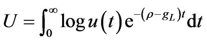
where  represents the instantaneous utility. The instantaneous utility function takes the form
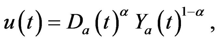
where  is traditional goods and
  a composite good of modern goods,
  where
where  is the expenditure share of the modern good while
  is the expenditure share of the traditional good.
  represents the subjective discount rate. The composite good of modern goods is given by
where is the number of varieties produced and
  is the consumption of the
  -th variety. The value of per-capita expenditure is given by
where
 is the price of the
  -th modern goods and
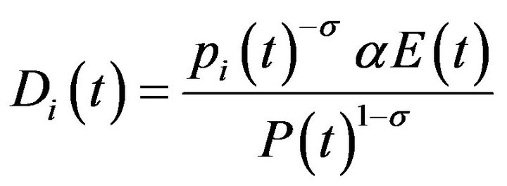
  the price of the traditional good. The individual demand for modern goods is
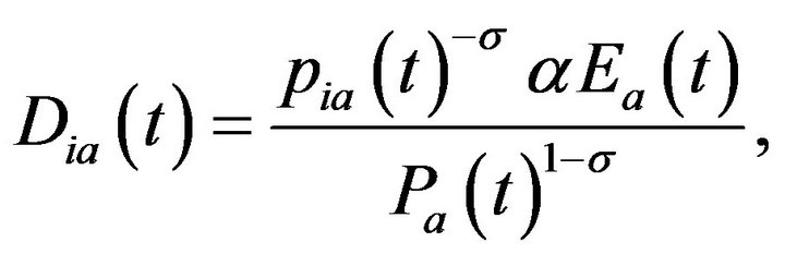
where
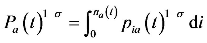
is the price index. The intertemporal budget constraint is given by
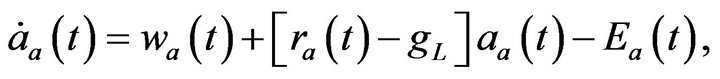
where  is per capita financial assets,
  the wage rate, and
  the market interest rate. The time path of per capita expenditure is determined by
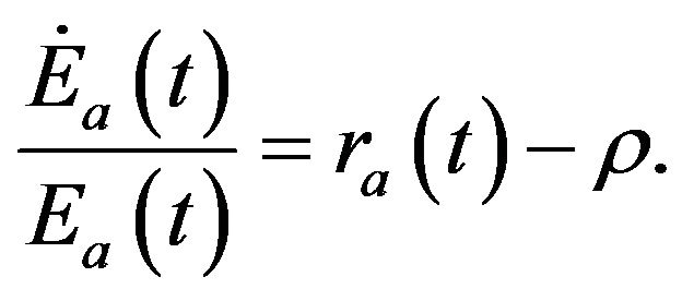
Our analysis focuses on the steady state with constant per capita expenditure. Thus, 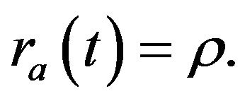
We turn to explaining the modern-good firm. Starting to produce a modern good requires one unit of capital (the perpetual patent which gives each innovator monopoly power). Thus, the total amount of capital must be fixed by the total number of varieties so that  The unit labor requirement associated with producing a modern good is
  Given aggregate expenditure and other firms’ prices, each firm maximizes its instantaneous profit by setting the profit-maximizing price. The profit-maximizing price is
The demand function for each variety is
The profit function for a modern good is
A traditional good is produced using only labor by a one-to-one technology. Thus, the aggregate demand for the traditional good is
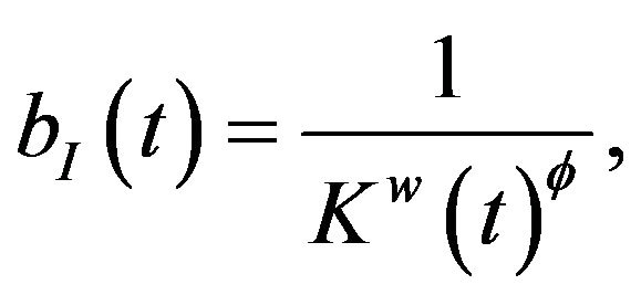
We now explain the R & D sector. This sector is characterized by free entry and perfect competition, and uses only labor as an input. We consider the case of local knowledge spillover. A unit labor requirement for creating capital (new variety) is given by
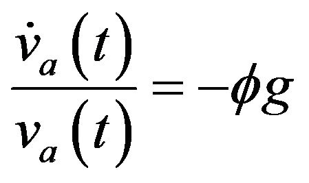
where  is the intertemporal knowledge spillover. The capital (new variety) evolves according to:
where  represents the total amount of R&D labor. The R & D sector is perfectly competitive and has constant returns to labor. The free entry condition is
  where
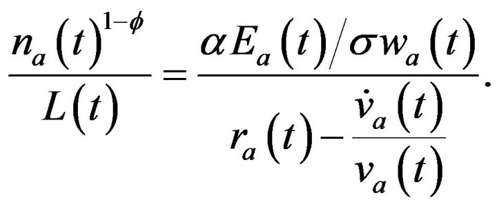
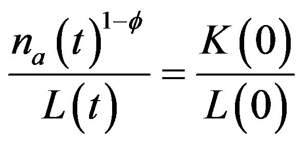
where  is the value of a modern good firm. In steady-state equilibrium,
 holds.
Saving takes the form of riskless bonds or shares of firms. The return on shares of firms comes from the dividend rate,
plus the capital gain (loss),
On the other hand, the return on the riskless bond is given by  Thus, the no-arbitrage condition is
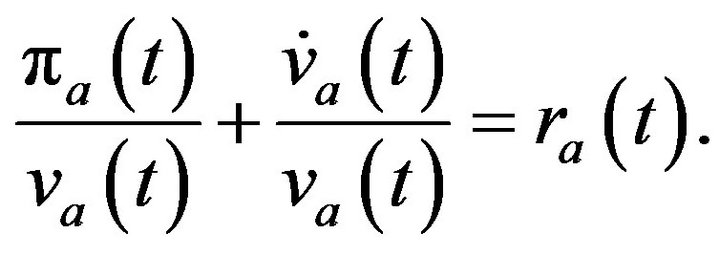
Inserting the profit function, free entry condition, and  into the no-arbitrage condition, it is rewritten as
Using the free entry condition, we derive
in the steady state. Moreover
from the fact that
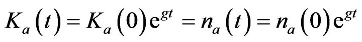 and
and 
Substituting these results into the no-arbitrage condition yield

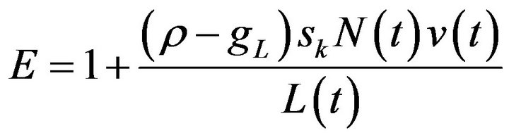
Using the no-arbitrage conditions, we get the gap in per capita expenditure as follows,
 (1)
(1)
The difference in per capita expenditure increases with the difference in capital stocks with elasticity  This is because the dividend rate depends positively on expenditures and negatively on the number of varieties with elasticity
  from the no arbitrage condition. Thus, there is a positive relationship between per capita expenditure and the wage rate. From the free entry condition, the intertemporal knowledge spillover reduces the value of capital, and thus per capita expenditure. When the intertemporal knowledge spillover, ϕ approaches 1, the difference in per capita expenditures between the two countries disappears. Notice that the fraction of labor devoted to the R & D sector is
and the fraction of labor devoted to manufacturing sectors is
and we need not consider the labor market constraint.
The difference in the price indexes between the two countries is given by:
 (2)
(2)
Notice that the gap between the price indexes3 depends on the difference in capital stock with elasticity

because the price index depends negatively on the number of varieties produced, and the number of varieties in each country equals the capital stocks which is raised to
When the elasticity of substitution between varieties
 approaches infinity, the difference in the price indexes between the two countries disappears because the number of varieties is not important for consumers and price indexes take the same values. Finally, using (1) and (2), the real income of Country A relative to Country B is:
 (3)
(3)
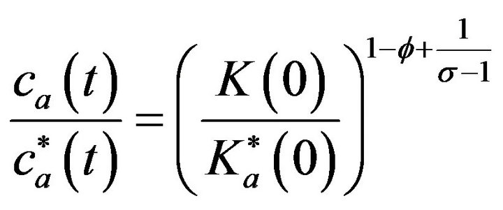
The real income in each country depends on per capita expenditure relative to the price index. Thus, autarkic regional inequality increases with regional difference in capital stocks since elasticity,
is non-negative When
When
autarkic regional inequality exists due to  When
When
autarkic regional inequality does not exist.
4. Open Economy
We follow Minniti and Parello [9]. There is international trade of traditional good which is freely traded and of modern goods which faces iceberg costs and of capital flow which is also freely traded and so interest rates, instantaneous profits, and the value of capital (patents) are equalized between the two countries. Notice that the only equilibrium we consider is that both countries produce the traditional good whose unit labor requirement and price are unity, and so wages are also unity. We assume international knowledge spillover in the R & D sector.
Instantaneous utility depends on the amount of consumption of the traditional good and modern goods, and the consumer has the following instantaneous utility function:  where
where is traditional goods and
  a quantitative index of modern goods,
  where
where is the expenditure share of the composite modern good and
  is the expenditure share of the traditional good. Consumer maximizes the intertemporal utility function
where  denotes the subjective discount rate and
  the population growth rate. The quantitative index of modern goods is specified by
where  denotes the total number of varieties produced in Country A,
  represents the number of varieties produced in Country B,
  is the amount of the
  -th variety produced and consumed in Country A, and
  the amount of the
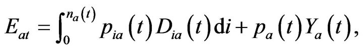
  -th variety produced in Country B and consumed in Country A. The individual expenditure takes the form
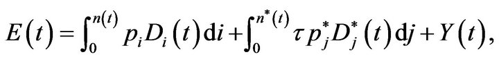
where indicates the producer price of modern goods produced in Country A,
  the producer price of modern goods produced in Country B, and
  the iceberg cost.
The individual demands for domestically-produced and imported varieties are obtained as
and 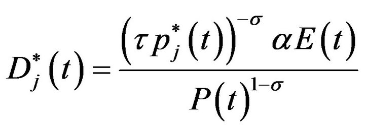
where
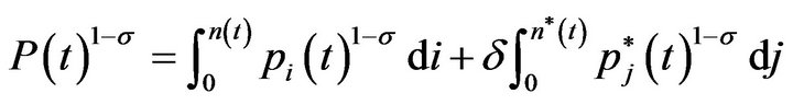
represents the price index and 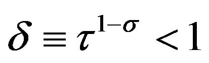 a measure of the freeness of trade. Per capita expenditure accumulates according to
where  is the international interest rate. For a firm to start to produce one modern good requires one unit of capital. Thus, the total amount of capital must be equal to the total number of varieties so that
  Moreover, producing
 units of a variety requires
  and
and  units of labor for serving domestic and foreign markets, respectively. Thus, the profit-maximizing producer prices are
the profit functions for each modern good are
The aggregate demand for home and foreign modern goods is
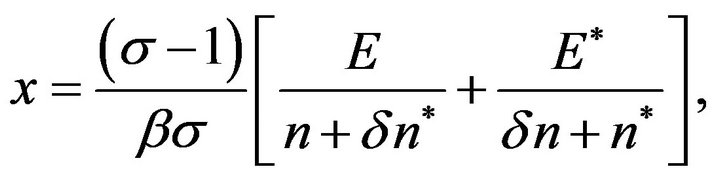
and
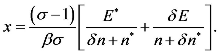
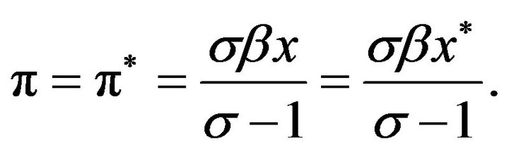
Although a worker cannot move between the two countries, firms can freely move between the two countries with zero costs. The instantaneous profits are repatriated to the region where the owner lives, and the instantaneous profits between the two regions must be equalized at each instant in time so that  Dividing both sides of the last condition by the world-wide expenditure,
  and the world-wide varieties
  to get
 where
where
represents Country A’s share of the economy-wide per capita expenditure and
denotes Country A’s share of total varieties produced.
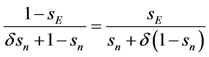
Rearranging the result, Country A’s share of  is derived as a function of Country A’s share of E and parameters as follows:
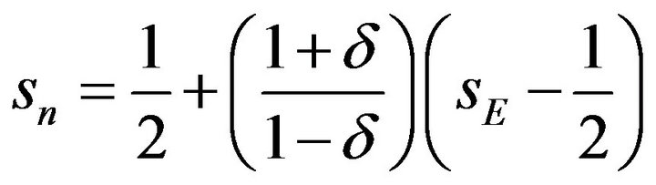 (4)
(4)
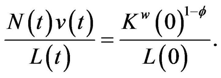
Using these results yields
The R & D sector4 is characterized by perfect competetion, free entry, and international knowledge spillover5. This sector uses only labor as a production factor. The unit labor requirement for variety creation is given by
where  measures the strength of the intertemporal knowledge spillover. The flow of new varieties is given by
where  is the total amount of labor employed in R & D. Free entry in the R & D sector implies
  In the steady-state equilibrium, we obtain
where
The return on shares of firms comes from the dividend rate and capital gains. Thus, the no-arbitrage condition on firm share is  After some manipulation, we get
This condition yields the demand for labor devoted to the R & D sector and the manufacturing sector.
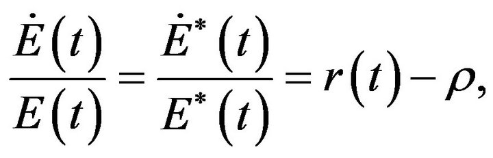
We next turn to examine regional income inequality. In the steady-state equilibrium per capita expenditure must be constant, which in turn implies  The inter-temporal budget constraints can be solved for
and
respectively. Using the free entry condition,  so
so
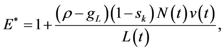
Thus, we represent the gap in expenditure per person between Country A and Country B as:
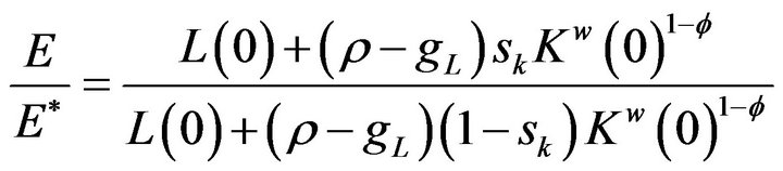 (5)
(5)
Moreover, the difference in per capita expenditure between the two countries depends on the difference in incomes which itself depends on their share of capital owned. The value of capital depends negatively on intertemporal knowledge spillover from the free entry condition. When the intertemporal knowledge spillover  approaches 1, the difference in per capita expenditure between the two countries shrinks, but does not disappear. This result differs from the closed economy. Using (4) and
  and
and  we get
where
measures the relatively higher Country A’s expenditure due to higher asset income. By substituting  into (4), Country A’s share of firms located is given by:
 (6)
(6)
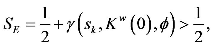
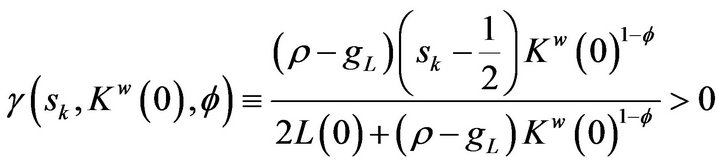
Notice that each consumer earns income from labor and financial assets. The former is the same across countries, but the latter is different across the two countries because
 This implies
  Moreover,
holds due to Country A’s higher aggregate demand, the existence of iceberg costs, and increasing returns in modern goods. When Country A’s share of  is large and the intertemporal knowledge spillover is small, Country A’s shares of
  and
and  are large. Even when the intertemporal knowledge spillover approaches 1,
 and
and 
By substituting profit-maximizing price and (6) into price index in Country A and Country B, We write the relative price index of Country A to Country B as
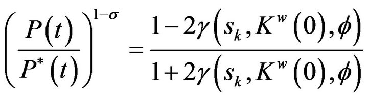 (7)
(7)
The difference in price indexes depends on the proportion of Country A’s firms located in Country A which itself now depends, through the difference in asset income, on the difference in per capita expenditures. When the elasticity of substitution between modern goods approaches positive infinity, the difference in price indices disappears.
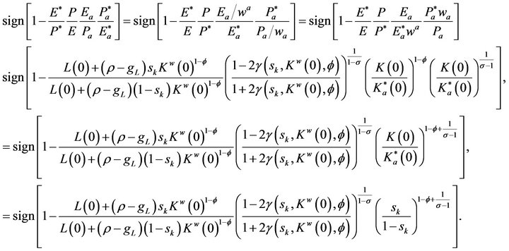
We finally turn to examine the effects of opening trade on regional inequality. Using (1), (2), (5), and (7), it6 is obtained as:
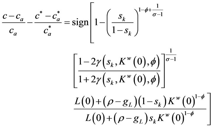 (7)
(7)
When the elasticity of substitution between varieties and inter-temporal knowledge spillover are (not) sufficiently large and Country A’s capital share is not too large (too large), regional inequality increases (decreases). The reason why regional inequality is increased is because when
and  the autarkic regional inequality is very low compared with regional inequality and, in other words, Country A’s per capita expenditure is higher than Country B’s per capita expenditure in the open economy as well as the levels of other components in the North is the same as other components in the County B. The reason why regional inequality is decreased is when
and  the level of autarkic Country A’s real income is sufficiently higher than Country B’s autarkic real income, that is, regional inequality in the closed economy is very high. This is not offset by the increase in the regional inequality in the open economy through agglomeration due to increasing returns in modern goods sector and iceberg costs.
5. Concluding Remarks
We show that opening trade on regional inequality can raise or reduce inequality in a semi endogenous growth model with foot-loose capital, local knowledge spillover in a closed economy, and also international knowledge spillover in an open economy. When regional inequality in a closed economy is sufficiently low (high), in other words, when each firm has a (not) sufficiently weak monopoly power in the modern sector and has a (not) sufficiently large inter-temporal spillover in R & D, and not sufficiently (sufficiently) large share of capital owned, opening trade has a positive (negative) effect on regional inequality in an economy with autarkic local knowledge spillover.
In this paper, we only consider the equilibrium in which the two countries produce homogenous goods. We can examine the effects of opening trade on international wage inequality as a natural extension by considering an equilibrium in which one country produces a traditional good.
6. Acknowledgements
The author thanks David Denslow, Elias Dinopoulos, Jonathan Hamilton, Takashi Kamihigashi, and Tamotsu Nakamura. This research was supported in part by a grant from Hisa Scholarship. The usual disclaimer applies. Much of the research reported here was done in the 2012, when Fukuda visited the University of Florida, whose hospitality he gratefully acknowledges.
REFERENCES
- G. Wan, M. Lu and Z. Chen, “Globalization and Regional Income Inequality: Empirical Evidence from within China,” Review of Income and Wealth, Vol. 53, No. 1, 2007, pp. 35-59. doi:10.1111/j.1475-4991.2007.00217.x
- C. Zhao and Y. Jin and M. Lu, “Economic Opening and Industrial Agglomeration in China,” In: M. Fujita, S. Kumagai and K. Nishikimi, Eds., Economic Integration in East Asia: Perspectives from Spatial and Neoclassical Economics, Edward Elgar Publishing Limited, Cheltenham, 2008, pp. 276-315.
- T. Jian, J. D. Sachs and A. M. Warner, “Trends in Regional Inequality in China,” China Economic Review, Vol. 7, No. 1, 1996, pp. 1-21. doi:10.1016/S1043-951X(96)90017-6
- R. Kosfeld and J. T. Lauridsen, “Dynamic Spatial Modeling of Regional Convergence Processes,” Empirical Economics, Vol. 29, No. 4, 2004, pp. 705-722. doi:10.1007/s00181-004-0204-x
- K. Behrens, J. H. Hamilton, G. I. P. Ottaviano and J. F. Thisse, “Commodity Tax Harmonization and the Location of Industry,” Journal of International Economics, Vol. 72, No. 2, 2007, pp. 271-291. doi:10.1016/j.jinteco.2006.08.002
- K. Behrens, J. H. Hamilton, G. I. P. Ottaviano and J. F. Thisse, “Commodity Tax Competition and Industry Location under the Destination and the Origin Principle,” Regional Science and Urban Economics, Vol. 39, No. 4, 2009, pp. 422-433. doi:10.1016/j.regsciurbeco.2009.01.008
- P. Martin and G. I. P. Ottaviano, “Growing Locations: Industry Location in a Model of Endogenous Growth,” European Economic Review, Vol. 43, No. 2, 1999, pp. 281-302. doi:10.1016/S0014-2921(98)00031-2
- P. Martin and G. I. P. Ottaviano, “Growth and Agglomeration,” International Economic Review, Vol. 42, No. 4, 2001, pp. 947-968. doi:10.1111/1468-2354.00141
- A. Minniti and C. P. Parello, “Trade Integration and Regional Disparity in a Model of Scale-Invariant Growth,” Regional Science and Urban Economics, Vol. 41, No. 1, 2011, pp. 20-31. doi:10.1016/j.regsciurbeco.2010.07.003
- E. Dinopoulos and P. Thompson, “Scale Effects in Schumpeterian Models of Economic Growth,” Journal of Evolutionary Economics, Vol. 9, No. 2, 1999, pp. 157-185. doi:10.1007/s001910050079
- C. I. Jones, “Growth and Ideas,” In: P. Aghion and S. N. Durlauf, Eds., Handbook of Economic Growth, NorthHolland, Amsterdam, 2005, pp. 1063-1111. doi:10.1016/S1574-0684(05)01016-6
- C. I. Jones, “R & D-Based Models of Economic Growth,” Journal of Political Economy, Vol. 103, No. 4, 1995, pp. 759-784. doi:10.1086/262002
- E. Dinopoulos and F. Sener, “New Directions in Schumpeterian Growth Theory,” In: H. Hanush and A. Pyka, Eds., Elgar Companion to Neo-Schumpeterian Economics, Edward Elgar Publishing Limited, Cheltenham, 2007, pp. 688-704.
- P. Segerstrom, “Endogenous Growth without Scale Effects,” American Economic Review, Vol. 88, No. 5, 1998, pp. 1290-1310.
- E. Dinopoulos and P. Thompson, “Schumpeterian Growth without Scale Effects,” Journal of Economic Growth, Vol. 3, No. 4, 1998, pp. 313-335. doi:10.1023/A:1009711822294
Mathematical Appendix
In this appendix, we derive Equation (7). We can rewrite
Furthermore,
We further rewrite this equation in a following way.
NOTES
1The two countries are the same except for the larger share of country A’s capital.
2See Dinopoulos and Thompson [10], Jones [11] and Dinopoulos and Sener [12] for survey articles about scale effects in the growth literature. See Jones [13] and Segerstrom [14] for a semi endogenous growth model and Dinopoulos and Thompson [15] for a fully endogenous growth model.
3The difference in price index represents the difference in price index relative to the wage rate in Country A and the price index in Country B.
4Due to international spillover and identical wage rate, R & D activity is conducted in two countries. The world production function for R & D is given by 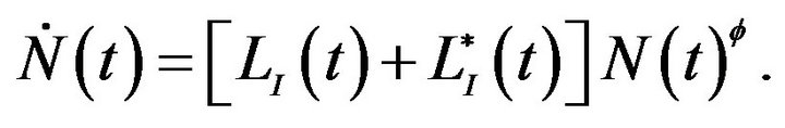
5The main results do not change when we assume local knowledge spillover.
6See Appendix for deriving Equation (7).