Journal of Mathematical Finance
Vol.06 No.01(2016), Article ID:63353,14 pages
10.4236/jmf.2016.61002
On the Stochastic Dominance of Portfolio Insurance Strategies
Hela Maalej1, Jean-Luc Prigent2
1ThEMA, University of Cergy-Pontoise, Boulevard du Port, France
2ThEMA and LabeX MME-DII, University of Cergy-Pontoise, Boulevard du Port, France

Copyright © 2016 by authors and Scientific Research Publishing Inc.
This work is licensed under the Creative Commons Attribution International License (CC BY).
http://creativecommons.org/licenses/by/4.0/


Received 27 October 2015; accepted 2 February 2016; published 5 February 2016
ABSTRACT
This paper compares the performance of the two main portfolio insurance strategies, namely the Option-Based Portfolio Insurance (OBPI) and the Constant Proportion Portfolio Insurance (CPPI). For this purpose, we use the stochastic dominance approach. We provide several explicit sufficient conditions to get stochastic dominance results. When taking account of specific constraints, we use the consistent statistical test proposed by Barret and Donald [1] . It is similar to the Kolmogrov- Smirnov test with a complete set of restrictions related to the various forms of stochastic dominance. We find that the CPPI method can perform better than the OBPI one at the third order stochastic dominance.
Keywords:
Stochastic Dominance, Portfolio Insurance, CPPI, OBPI, Barret and Donald Test

1. Introduction
The goal of portfolio insurance is to provide a guarantee against portfolio downside risk (usually 100% of the initial invested amount) while allowing to benefit from significant gains for bullish markets. The two standard portfolio insurance methods are the Option Based Portfolio Insurance (OBPI), introduced by Leland and Rubinstein [2] and the Constant Proportion Portfolio Insurance (CPPI) considered by Perold [3] . Basically, the OBPI portfolio is a combination of a risky asset S (usually a financial index such as the S&P) and a put written on it. Whatever the value of S at the terminal date T, the portfolio value will be always higher than the strike of the put. Therefore this strike is chosen in order to provide the desired guaranteed level. The standard CPPI method consists in a simplified strategy to allocate assets dynamically over time. A floor is initially determined such as it is equal to the lowest acceptable value of the portfolio. Then, the amount allocated to the risky asset (called the exposure) is defined as follows: the cushion, which is equal to the excess of the portfolio value over the floor is multiplied by a predetermined multiple. The remaining funds are usually invested in the reserve asset, usually T-bills. As the cushion approaches zero, exposure approaches zero too. In continuous time, this keeps portfolio value from falling below the floor.
To compare these two main portfolio strategies, we search for stochastic dominance (SD) properties since SD takes account of the entire return distribution. The major argument for stochastic dominance is that it does not require any specific knowledge about the preferences of investors. Indeed, the first stochastic dominance order is related to investors with an increasing utility function. Stochastic dominance of order two focuses on investors having an increasing and concave utility, meaning that they are risk-averse1. However, at a given order (for example 1 or 2), the stochastic dominance criterion cannot always allow to rank all portfolios. There exist cases where no stochastic dominance is observable. But there exists a stochastic dominance criteria at each order and, the higher the order, the less stringent the criterion. Thus it is reasonable to expect that there exists an order for which a portfolio strategy dominates another one (or vice versa). De Giorgi [6] shows that, in a market without friction, the market portfolio can be efficient according to the criterion of the second order stochastic dominance. Therefore the test of stochastic dominance is consistent with the theory of portfolio choice. To compare with alternative approaches such as those based on performances measures, note that Darsinos and Satchell [7] show that n-order stochastic dominance implies Kappa (n − 1) dominance. It means for example that the second order stochastic dominance implies the Omega dominance while the third order SD implies dominance according to the Sortino measure.
For the portfolio insurance strategies, Bertrand and Prigent [8] proved that the stochastic dominance at the first order is a too strong condition, meaning that neither the CPPI nor the OBPI dominates the other strategy for this criterion2. However, as proved theoretically by Zagst and Kraus [10] , stochastic dominance of portfolio insurance strategies can be obtained mainly from the third order. Our main purpose is to extend previous results when taking account of quite general share values and/or of specific constraints such as capped strategies introduced to limit financial risk exposures.
The paper is organized as follows. In Section 2, we briefly introduce the basic properties of the CPPI and the OBPI strategies. In Section 3, we examine the stochastic dominance (SD) framework to compare portfolio insurance strategies. First, we provide several sufficient conditions to get stochastic dominance properties for the standard portfolio insurance methods. Second, to extend previous results, we introduce specific statistical tests and simulation methods for computing p-values when examining SDj with j larger than one. We use the test considered by Barret and Donald [1] , based on the multiplier central limit theory discussed in Van der Vaart and Wellner [11] .
2. Basic Properties of the CPPI and the OBPI Strategy
2.1. The Financial Market
We consider two basic assets that are traded in continuous time during the investment period . The “risk-free” asset (a money market account for example) is denoted by B. Denote by r the constant continuous interest rate
 . We get:
 (1)
(1)
with initial value . The risky asset (for example a financial market index) is denoted by S. It is assumed to be a geometric Brownian motion given by:
 (2)
(2)
with non negative initial value  and where
  is a standard Brownian motion. There exists
a constant drift term parameterized by  and a volatility denoted by
 .
.
To price options, we use the Black and Scholes formula while taking account of the spread between the empirical and the implied volatility3.
2.2. Constant Proportion Portfolio Insurance (CPPI)
The standard CPPI method consists in a simplified strategy to allocate assets dynamically over time so that its value  never falls below the floor
 . This latter one is equal to the lowest acceptable value of the portfolio and is defined as a percentage p (
 ) of the initial investment
 , i.e.:
 (3)
(3)
The excess of the portfolio value over the floor is called the cushion . It is equal to:
 (4)
(4)
Then, the amount allocated on the risky asset (called the exposure ) is equal to the cushion multiplied by a constant multiple m. Therefore, the exposure
  satisfies:
 (5)
(5)
The interesting case is when , that is when the payoff function of the portfolio value at maturity
  is a convex function with respect to the risky asset
 .
.
Then the cushion value  must satisfy:

By applying Itô’s lemma, we obtain:
 (6)
(6)
By using the relation:

we deduce:

Substituting this expression for  into the expression for
  leads to:
 (7)
(7)
with

We deduce that the value of the CPPI portfolio  at any time t is given by:
 (8)
(8)
Note that, for the CPPI method, the two key management parameters are the initial floor value  and the multiple m.
Remark 2.1. (Capped CPPI) The manager may want to increase his profits, from usual performances of asset S while potentially discarding very high values of S. In that case, the exposure is determined by:
 (9)
(9)
where  denotes the gearing coefficient. Its usual value is equal to 0.9.
2.3. Option-Based Portfolio Insurance (OBPI)
In what follows, we describe the option-based portfolio insurance strategy. It provides a guarantee equal to whatever the market fluctuations. Indeed, for a given share q, we have:
 (10)
(10)
which implies that  if
if .
.
This relation shows that the insured amount at maturity is the exercise price multiplied by the number of shares, i.e. . The value
  of this portfolio at any time t in the period
  is equal to:

where  denotes the Black-Scholes value of the European call option with strike K, calculated under the risk neutral probability Q.
The portfolio value , for all dates t before T, is always above the deterministic level
 . In order to guarantee the minimum terminal portfolio value
 , the strike K of the European Call option must satisfy the following relation:

which implies that:
 (11)
(11)
Therefore, the strike K is an increasing function  of the percentage p, since in Equation (Equation (11)) both functions are decreasing respectively with respect to K and p. Then, the number of shares q is given by:
 (12)
(12)
Thus, for any investment value , the number of shares q is a decreasing function of the percentage p.
In what follows, we price the option using the implicit volatility .
.
We denote its price by .
.
Remark 2.2. (Capped OBPI) If the manager wants to increase his profit while potentially discarding very high value of S, the options are capped at a level L, as follows. Consider a parameter L higher than the strike K.
The terminal value of the capped OBPI with strike K and parameter L is defined by:
 (13)
(13)
3. Stochastic Dominance of Portfolio Insurance Strategies
3.1. Stochastic Dominance: Theoretical Results
In what follows, we provide several sufficient conditions to get stochastic dominance results as in Zagst and Kraus [10] but without assuming as them that q is equal to 1 (see previous Relation 12).
3.1.1. The Second Order Stochastic Dominance
Mosler [12] has stated a theorem for determining the second order stochastic dominance (denoted by ) between random variables based on the condition of intersection between the cumulative distribution functions.
Theorem 3.1. (Mosler [12] ). Let  and V be two random variables with finite expectations. Denote for all
 ,
,  the difference of their respective cumulative distributions functions. Then, we get:

where  denotes the set of all real functions H, with k changes of sign:

We deduce that, if , then the two functions
  and
and  intersect k times.
For example, we have:

And

The second order stochastic dominance depends on the values taken by the multiple m, the historical volatility  and the implied volatility
  used to price the Call for the OBPI strategy. The determination of the second order stochastic dominance requires understanding the behavior of the function
  based on the values taken by the multiple m. If
 , then the function H is strictly decreasing and presents a single point of intersection with the horizontal axis, thus
 . Therefore, for
 ,
,  , we can conclude,
using theorem of Mosler [12] , that, if  and
and , then the CPPI strategy stochasti- cally dominates at the second order the OBPI strategy.
Theorem 3.2. Let  and
and . Additionally, assume that
 . Then, we deduce:

Proof. See Appendix A1.
Remark 3.1. Condition  insures that
  which allows proving the previous theorem. When
  (as in Zagst and Kraus [10] ), this condition is necessary satisfied.
3.1.2. The Third Order Stochastic Dominance
As mentioned by Zagst and Kraus [10] , the third order stochastic dominance (denoted by ) can be deduced under some specific assumptions.
Theorem 3.3. (Karlin-Novikov; Mosler [12] )
Let ,
,  be non-negative random variables with finite second moments.
Denote  for all
  Then:
Then:

The validation of the third order stochastic dominance requires the analysis of the condition  of previous Karlin and Novikov theorem. We get:
Theorem 3.4. Assuming that , there exists a value
  of the multiple such that:

Proof. See Appendix A.2.
Using previous theorems, we deduce:
Theorem 3.5. Let  defined by:

and .
.
Then, we get:

Proof. Condition  implies that
  (see Appendix A.1) while condition m ≤
mmax implies that . Therefore, using Karlin and Novikov theorem, we deduce the result.
To illustrate these theoretical results, we consider the following numerical example: ,
,  ,
,  ,
,  ,
,  ,
,  , and
, and . Applying Relation (11), we deduce that
  and
and . Table 1 illustrates the results of the third degree stochastic dominance for different values of the multiple
 .
.
Results of Table 1 show third order stochastic dominance of the CPPI strategy for .
.
Recall that, if the multiplier , we have
 . However, for m ≥ mmax = 3.12,
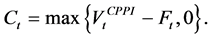
we have  and the sufficient condition of Karlin and Novikov theorem is no longer satisfied. The range of the multiple values, for which a stochastic dominance at the third order is verified, depends notably on the values of the implied volatility, the empirical volatility and the drift. Figures 1-3 illustrate this dependence.

Table 1. The third order stochastic dominance for multipliers equal to 1, ∙∙∙, 5.
Figure 1. The value of mmin depending on the drift and the implied volatility.
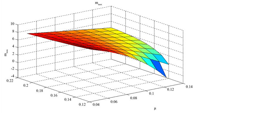
Figure 2. The value of mmax depending on the drift and the implied volatility.
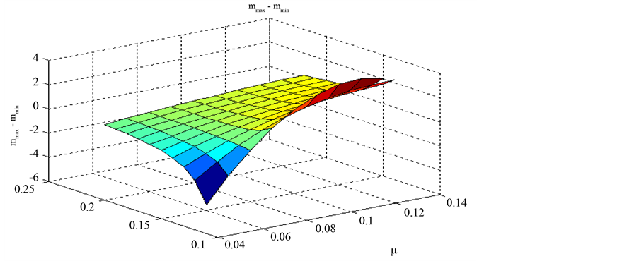
Figure 3. Difference of the upper and lower bounds on the multiplier.
The value of the lower bound  is a decreasing function with respect to the value of the drift
 . Indeed, when the drift increases, the expectation of the CPPI portfolio value increases more than that of the OBPI portfolio since the CPPI strategy is more allocated on the risky asset. The value of the lower bound
  is not always an increasing function of the implied volatility.
The value of the upper bound  is a decreasing function with respect to the value of the drift
 . Indeed, when the drift increases, the expectation of the square of the CPPI portfolio value increases more than that of the OBPI portfolio since the CPPI strategy is more allocated on the risky asset. Therefore, the condition
 is more stringent when the multiple m increases. The value of the lower bound
is almost always an increasing function of the implied volatility.
Previous stochastic dominance results have been established for the standard cases, i.e. the strategies are not capped. To deal with capped strategies as defined in Remarks (Capped CPPI) and (Capped OBPI), we have to conduct a numerical analysis. In a first step, we simulate the portfolios values using standard Monte Carlo methods; in a second step, we test the stochastic dominance properties.
4. Stochastic Dominance of Portfolio Insurance Strategies
4.1. Stochastic Dominance: Numerical and Empirical Tests
In the empirical framework, the stochastic dominance has been pioneered for example by Kroll and Levy [13] . To avoid sampling errors due to i.i.d. assumptions, general stochastic dominance tests have been developed (e.g. Davidson and Duclos [14] ; Barrett and Donald [1] ; Post [15] ; Linton et al. [16] ; Scaillet and Topaloglou [17] ). The tests introduced by Barrett and Donald [1] and Linton et al. [16] are based on a comparison of the cumulative density functions of studied perspectives. They are based on the Kolmogorov-Smirnov type tests. Barrett and Donald [1] examine the application of tests for any predetermined orders of stochastic dominance,  , using several simulation and bootstrap methods to estimate an asymptotic p-value.
4.1.1. Stochastic Dominance and Hypothesis Formulation
Due to the characterizations of stochastic dominance, it is convenient to represent the various orders of stochastic dominance using the integral operators,  , corresponding to successive integrations of the cumulative distribution function G to order
 , namely:


and so on.
The general hypotheses for testing stochastic dominance of G with respect to F at order j can be written compactly as:


4.1.2. Test Statistics and Asymptotic Properties
In this paper, we test for stochastic dominance using the empirical distribution functions estimated from simulation of the two insurance portfolio strategies. The test of Linton et al. [16] allows for dependence in the data, and can be conducted with a limited number of assumptions. Suppose two prospects X and Y. Let N be the number of the realizations for the two prospects  and
and . The null hypothesis is that a particular prospect X dominates the other one.
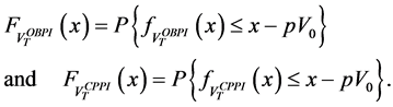
The empirical distributions used to construct the tests are respectively given by:
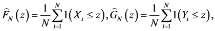
where j denotes the order of dominance and  denotes the indicator function.
The statistical test  for the full sample is defined by:

The linear operator  is written as:

The second term of the linear operator is derived from Davidson and Duclos [14] .
We have also to define a method in order to obtain the critical value of the test. The standard bootstrap does not work because we need to impose the null hypothesis in that case, which is difficult because it is defined by a complicated system of inequalities. According to Linton et al. [16] , we apply the sub sampling method which is very simple to define and yet provide consistent critical values. Following the circular block method of Kläver [18] , we have to compute again the test statistic for the sub sample of size b for each of the  different
subsamples , where
  and
and , and for the subsamples
 where
where . Let
. Let  be equal to the statistic
  evaluated at
the subsample  of size b. We have:

with

The underlying rationale is that one can approximate the sampling distribution of  using the distribution of the values of
  computed over
  different subsamples of size b, when
  and
and  as
as .
.
We consider that each of these sub samples is also a sample of the true sampling distribution of the original data.
Following Kläver [6] , we consider a sub sample size 
Let  denote the empirical p-value:

For , we reject the null hypothesis at
  significance according to the following rule:
・ If  we reject the null hypothesis of j-order stochastic dominance of variable X with respect to the variable Y.
・ If  the variable X stochastically dominates the variable Y at the j-order.
4.1.3. Numerical Illustrations
In this subsection, we apply the tests of stochastic dominance in particular to check if the interval  provided for the third order stochastic dominance between the CPPI strategies and OBPI strategies in previous theoretical subsection can be enlarged. We consider the case of a guarantee equal to 100% of the initially invested amount. Our numerical base case corresponds to a drift equal to 4.5%, an investment horizon equal to 8 years, an historical volatility equal to 15%. Our goal is to determine an order of stochastic dominance between the two insured portfolios by varying the multiplier of the CPPI strategy into the interval
 . We begin by varying the implicit volatility in
  as illustrated in Table 2.
We note that, for all cases in which the implied volatility far exceeds the historical volatility, the CPPI strategy, with a multiplier equal to 2, dominates the OBPI one.
We can also study the effect of the drift on the third order stochastic dominance (values of drift ). We still fix the investment maturity to 8 years and consider a historical volatility equal to15%, a multiplier range in
 , an implied volatility in
  and a guarantee level equal to 100%.
As shown in Table 3, the TSD is never verified, even if  and
and  when
when . We note that the CPPI strategy loses its attractiveness. Since
 , we conclude that the CPPI strategy takes less advantage from the trend increase.
For lower trend levels and implicit volatility  higher than the historical one
 , we get results given in Table 4.
Table 2. Third order stochastic dominance according to implicit volatility.
Table 3. No third order stochastic dominance cases.
Table 4. Third order stochastic dominance (low trend).
Remark 3.2. To summarize the numerical results:
-We have found that the CPPI method third order stochastically dominates the OBPI one for high implied volatility relatively to the empirical volatility;
-When the interval  degenerates, we can find multiples for which the CPPI is stochastically dominated at the third order by OBPI;
-The implied volatility interval where the dominance relation is insured is larger for high values of implied volatility, for low values of the drift and for high values of the multiple.
-The TSD property of the CPPI strategy is rejected for the low values of  with respect to
 .
.
-Through this numerical study, we can detect cases of third order stochastic dominance beyond the theoretical cases.
-Finally, when strategies are capped, the TSD property is generally not satisfied4.
5. Conclusion
In the present paper, we have compared the CPPI and OBPI strategies, mainly with respect to the third stochastic dominance (TSD). We find that the CPPI method third order stochastically dominates the OBPI one for high implied volatility relatively to the empirical volatility. We have checked the TSD of the CPPI method compared to the OBPI method for low values of the drift weighted by high values of the multiplier. We have shown that the relation of SDT is rejected for the low values of the implicit volatility with respect to the statistical one. Further extensions could be based on the use of almost stochastic dominance as defined by Leshno and Levy [19] , in order to extend the range of the multiple for which the CPPI dominates the OBPI.
Cite this paper
HelaMaalej,Jean-LucPrigent, (2016) On the Stochastic Dominance of Portfolio Insurance Strategies. Journal of Mathematical Finance,06,14-27. doi: 10.4236/jmf.2016.61002
References
- 1. Barrett, G.F. and Donald, S.G. (2003) Consistent Tests for Stochastic Dominance. Econometrica, 71, 71-104.
http://dx.doi.org/10.1111/1468-0262.00390 - 2. Leland, H.E. and Rubinstein, M. (1976) The Evolution of Portfolio Insurance. In: Luskin, D.L., Ed., Portfolio Insurance: A Guide to Dynamic Hedging, Wiley.
- 3. Perold, A. (1986) Constant Portfolio Insurance. Working Paper, Harvard Business School.
- 4. Levy, H. (1992) Stochastic Dominance and Expected Utility: Survey and Analysis. Management Science, 38, 555-593.
http://dx.doi.org/10.1287/mnsc.38.4.555 - 5. Levy, H. (2015) Stochastic Dominance: Investment Decision Making under Uncertainty. 3rd Edition, Springer-Verlag.
- 6. De Giorgi, E. (2005) Reward-Risk Portfolio Selection and Stochastic Dominance. Journal of Banking and Finance, 29, 895-926.
http://dx.doi.org/10.1016/j.jbankfin.2004.05.027 - 7. Darsinos, T. and Satchell, S. (2004) Generalizing Universal Performance Measures. Risk, 17, 80-84.
- 8. Bertrand, P. and Prigent, J.-L. (2005) Portfolio Insurance Strategies: OBPI versus CPPI. Finance, 26, 5-32.
- 9. Prigent, J.-L. (2007) Portfolio Optimization and Performance Analysis. Chapman & Hall, Boca Raton.
http://dx.doi.org/10.1201/9781420010930 - 10. Zagst, R. and Kraus, J. (2011) Stochastic Dominance of Portfolio Insurance Strategies: OBPI versus CPPI. Annals of Operations Research, 185, 75-103.
http://dx.doi.org/10.1007/s10479-009-0549-9 - 11. Van Der Vaart, A.W. and Wellner, J.A. (1996) Weak Convergence and Empirical Processes with Applications to Statistics. Springer-Verlag, New York.
http://dx.doi.org/10.1007/978-1-4757-2545-2 - 12. Mosler, K.-C. (1982) Entscheidungsregeln bei Risiko-Multivariate stochastische Dominanz. Springer, Heidelberg.
http://dx.doi.org/10.1007/978-3-642-95419-1 - 13. Kroll, Y. and Levy, H. (1980) Sampling Errors and Portfolio Efficient Analysis. Journal of Financial and Quantitative Analysis, 15, 655-688.
http://dx.doi.org/10.2307/2330403 - 14. Davidson, R. and Duclos, J.-Y. (2000) Statistical Inference for Stochastic Dominance and for the Measurement of Poverty and Inequality. Econometrica, 68, 1435-1464.
http://dx.doi.org/10.1111/1468-0262.00167 - 15. Post, T. (2003) Empirical Tests for Stochastic Dominance. Journal of Finance, 58, 1905-1932.
http://dx.doi.org/10.1111/1540-6261.00592 - 16. Linton, O., Maasoumi, E. and Whang, Y.-J. (2005) Consistent Testing for Stochastic Dominance under General Sampling Schemes. Review of Economic Studies, 72, 735-765.
http://dx.doi.org/10.1111/j.1467-937X.2005.00350.x - 17. Scaillet, O. and Topaloglou, N. (2010) Testing for Stochastic Dominance Efficiency. Journal of Business & Economic Statistics, 28, 169-180.
http://dx.doi.org/10.1198/jbes.2009.06167 - 18. Kläver, H. (2005) Testing for Stochastic Dominance Using Circular Block Methods. Graduate School of Risk Management, University of Köln.
- 19. Leshno, M. and Levy, H. (2002) Preferred by All and Preferred by Most Decision Makers: Almost Stochastic Dominance. Management Science, 48, 1074-1085.
http://dx.doi.org/10.1287/mnsc.48.8.1074.169
Appendix
Appendix A.1. (Proof of Theorem 3.2)
The proof is similar to the proofs of Theorems 2, 3 and 4 of Zagst and Kraus [10] except that we take account of Relation (12)5.
-The first step consists in proving the following equivalence:

which is also equivalent to:

The proof is straightforward, using usual computations of both  and
and . Note this condition does not depend on q.
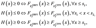
-The second step is to demonstrate that, for , the function
  satisfies the following property:

For this purpose, we can note that both the cumulative functions  and
and  can be written as follows:


Therefore, we deduce in particular that the sign of H does change on  since
since .
.
For , we have to prove that the sign of H changes exactly twice. Therefore, we search the solutions of the equation
 . Denote:

Then we get:
Therefore,  and
and  intersect if and only
  and
and  does, which is equivalent to

Now, we introduce the function .
.
1) For , it reaches a minimum at a given value
 .
.
Therefore, if  the function h has exactly two zeros
  and
and , which means that
  and
and  intersect twice.
Standard calculus leads to the following condition:

In that case, we have:
which implies that .
.
2) For , there exists only one intersection point equal to
  provided that
 .
.
This latter condition is equivalent to . It is necessary satisfied for the special case
  of Zagst and Kraus [10] . It implies that
 .
.
Appendix A.2. (Proof of Theorem 3.4)
The proof is similar to the proof of Theorem 6 of Zagst and Kraus [10] but it takes account of Relation (12).
We have to examine the condition .
.
-For the CPPI strategy, we get:

-For the OBPI strategy, we get:

and


with  and
and .
.
Then, we get:

from which we deduce:


We have also:

which obviously does not depend on the multiple m.
Introduce now the function g defined by:

The function  is continuous and strictly increasing. It converges to infinity when m goes to infinity.
Therefore, assuming that , there exists one and only one value
  such that
Finally, we deduce that:

Note that condition  is equivalent to
  since, for
 , the CPPI strategy
corresponds to a whole investment on the risk free asset B.
NOTES

1See Levy ( [4] [5] ) for details about stochastic dominance and expected utility, with applications to investment strategies.
2For details about various comparisons of CPPI and OBPI strategies, see Prigent [9] .

3We consider that the two strategies operate in different market environments. While the CPPI strategy operates on the financial market with its empirical market volatility (the so-called “local volatility”), the OBPI uses options that have to be priced using the implied volatility. In the financial market, we observe a spread between the empirical volatility and the implied volatility corresponding to the usual “smile” effect.

4Numerical details available on request.

5More details are available on request.